
Cloud Computing (4): Cloud Storage Systems and Distributed Architecture
From CAP theorem to S3, HDFS, and Ceph -- a deep tour of distributed storage primitives, consistency, replication, erasure coding, and cost optimisation.

When Netflix stores petabytes of video, when Instagram serves billions of photos, when a quant fund replays a year of market data in minutes — behind every one of these workloads is a distributed storage system. Storage looks deceptively simple from a developer’s window (PUT key, GET key), but the moment you cross the boundary of a single machine, you inherit a stack of problems that has driven decades of research: how to survive disk failures, how to scale linearly, how to provide a consistency model that does not surprise the application, and how to do all of this while paying cents per gigabyte rather than dollars.
This article walks the entire stack: the theoretical floor (CAP, consistency, consistent hashing), the three storage shapes (object, block, file), the production systems you will actually use (S3, HDFS, Ceph), and the engineering levers (replication, erasure coding, lifecycle, multipart uploads) that turn raw capacity into a service-level guarantee.
What You Will Learn#
- The trade-off space — CAP, PACELC, and why partition tolerance is mandatory
- The three shapes of cloud storage — block, file, object: when each is the right primitive
- Object storage internals — partitioning, placement, durability, the request path through S3
- Distributed file systems — HDFS (master-based) vs Ceph (CRUSH peer-to-peer)
- Replication vs erasure coding — the math behind 11-nines durability at 1.5x overhead
- Operational design — consistency models, quorum, multipart uploads, lifecycle policies
- Cost engineering — storage classes, compression, deduplication, tiering policies
Prerequisites#
- Comfort with Python and a Unix shell
- Working mental model of TCP, HTTP, and a filesystem
- Parts 1-2 of this series (fundamentals and virtualisation) are recommended
The shape of the problem#
Why distributed storage is hard#
A single SSD can deliver hundreds of thousands of IOPS and survive years. The problem is that one of anything in production is a liability:
- A single disk dies every few years — in a fleet of 10,000, you replace one or more every day.
- A single machine is a capacity ceiling: you cannot grow past its rack slot or PSU budget.
- A single network path is a SPOF: one ToR switch reload takes the box dark.
So we replicate. The moment we replicate, we hit two deeper problems: keeping the copies in agreement (consistency), and keeping the service usable when the network splits the copies into islands (partitions). That is the territory the CAP theorem maps out.
Object vs Block vs File: pick the right primitive#
Before we get to consistency theory, fix the vocabulary. There are three storage shapes, and almost every cloud product is one of them in disguise:
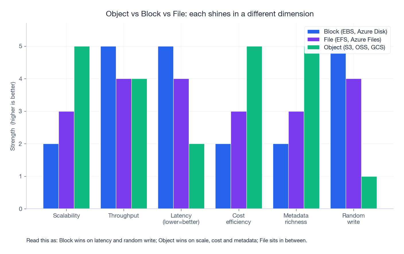
| Shape | Unit of access | API | Latency | Scale | Typical product | Best for |
|---|---|---|---|---|---|---|
| Block | 512 B / 4 KB blocks | iSCSI, NVMe, virtio | µs - low ms | TB per volume | EBS, Azure Disk, OSS-disk | Databases, VM root disks, anything wanting O_DIRECT |
| File | byte stream in a tree | NFS / SMB / POSIX | low ms | PB per fs | EFS, Azure Files, NAS | Shared scratch, lift-and-shift legacy apps |
| Object | immutable blob with metadata | HTTP/REST | tens of ms | exabytes | S3, GCS, OSS | Web assets, backups, data lakes, ML datasets |
A useful mental shortcut: block storage is a sector, file storage is a path, object storage is a URL. Each layer trades latency for scale. Block storage gives you a virtual disk (and the kernel gives you a filesystem on top). File storage gives you a shared filesystem out of the box. Object storage gives up POSIX semantics entirely in exchange for near-infinite scale and a flat key space.
When in doubt: if the workload is “open the file, seek, write” you want block or file. If it is “upload, download, delete by key” you want object.
CAP, PACELC, and the consistency menu#
The CAP theorem#
Eric Brewer’s CAP conjecture (2000), later proved by Gilbert and Lynch (2002), states: in the presence of a network partition, a distributed system must choose between Consistency and Availability. You cannot have both.
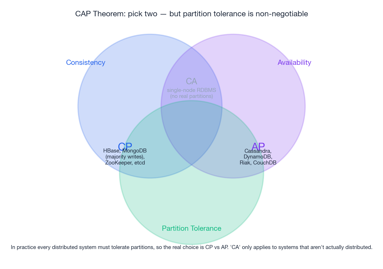
- Consistency (C) — every read returns the most recent committed write (linearisable).
- Availability (A) — every non-failing node returns a response in finite time.
- Partition tolerance (P) — the system continues to operate even when arbitrary messages between nodes are dropped.
Because partitions are not optional in a real network — a switch reload, a fibre cut, a kernel pause — you do not get to opt out of P. So the real choice is CP vs AP. “CA” describes single-machine systems that pretend partitions cannot happen.
| System | Class | Behaviour during a partition |
|---|---|---|
| ZooKeeper, etcd, HBase, MongoDB (majority writes) | CP | Refuse writes on the minority side; the cluster pauses but never disagrees |
| Cassandra, DynamoDB, Riak, S3 (legacy overwrite) | AP | Both sides keep accepting writes; reconciliation happens later |
| Single-node Postgres | CA-ish | Stops working entirely on partition (the partition is “the network is down”) |
PACELC: the part CAP forgot#
CAP only describes behaviour during a partition. PACELC (Abadi, 2010) extends it: if Partitioned, choose A or C; Else, choose Latency or Consistency.
This explains why Cassandra is “AP/EL” (eventual reads in normal operation are faster) while Spanner is “CP/EC” (it pays a TrueTime delay on every commit to stay strict). Most production decisions are PACELC decisions, not CAP decisions; partitions are rare but the latency-vs-consistency knob is set on every request.
Practical consistency models#
| Model | Guarantee | Where you see it |
|---|---|---|
| Linearisable | All operations appear in a single global order matching real time | etcd, Spanner, ZooKeeper |
| Sequential | Single global order, but not necessarily real time | classic shared memory |
| Read-after-write | A client always sees its own writes | S3 (since Dec 2020), most session-scoped systems |
| Monotonic reads | Once a client sees value v, it never sees an older value | Common in caches with sticky sessions |
| Eventual | If writes stop, reads eventually converge | Cassandra default, DynamoDB eventually-consistent reads |
S3’s switch to strong read-after-write consistency for all operations in December 2020 is a striking example of how engineering can collapse what looks like a fundamental trade-off: AWS rebuilt the metadata layer (an internal service called witness) to give linearisable behaviour without sacrificing the AP nature of the data path.
Consistent hashing: the routing primitive#
Sharding by hash(key) % N works until you add or remove a node, at which point (N -> N+1) reshuffles essentially every key. Consistent hashing (Karger et al., 1997) reduces the churn to roughly 1/N of keys. It is the placement algorithm beneath DynamoDB, Cassandra, Riak, memcached clients, and (with refinements) Ceph’s CRUSH.
The trick: hash both keys and nodes onto the same circular ring; each key is owned by the next node clockwise. Adding a node only steals keys from its immediate clockwise neighbour. Using virtual nodes (each physical node hashed multiple times) smooths the load distribution.
| |
Why 128 vnodes? With 1 vnode per server you get standard-deviation in load of ~30%. With 128 vnodes, the variance drops to a few percent — close enough to uniform that you can plan capacity by averages.
Object storage: how S3 actually works#
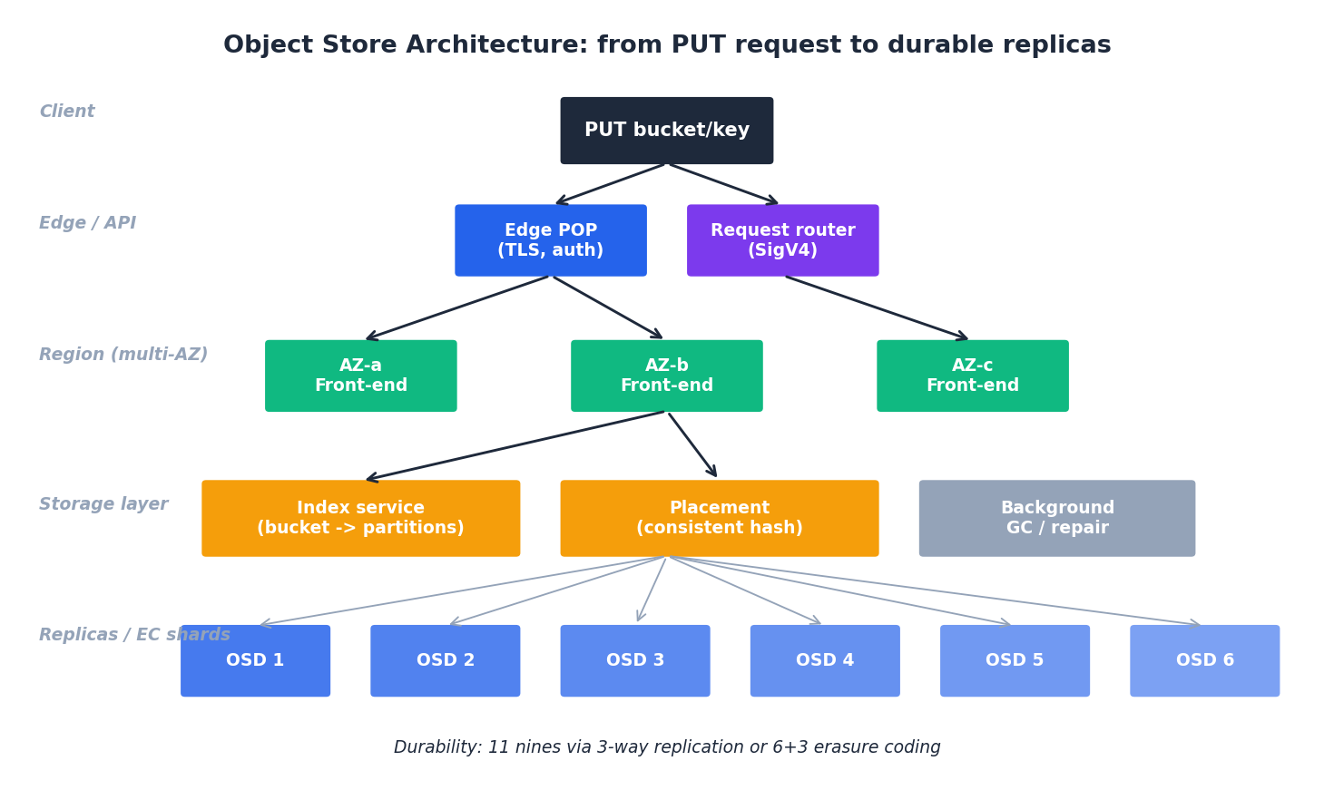
S3 is the de facto standard for cloud object storage and the inspiration for OSS, GCS, R2, Backblaze B2 and dozens of compatible systems. From a 30,000-foot view, S3 is “an HTTP server that maps (bucket, key) to bytes”. Inside, it is one of the largest distributed systems ever built.
The request path#
A PUT for s3://my-bucket/users/42.jpg:
- DNS + edge — the client resolves the regional endpoint and lands at an edge front-end.
- Auth — SigV4 signature is verified; bucket ACL / IAM policy / SCP / VPC endpoint policy / object ACL are evaluated.
- Index lookup — the bucket name maps to a partition of an internal key-range index. Hot buckets are auto-split (S3 will split a partition once it exceeds an internal QPS or size threshold; this is the historical reason for the “key prefix randomisation” advice, which is now mostly obsolete).
- Placement — the placement service picks an OSD set in the target durability scheme (e.g. 6+3 erasure coding spread across 3 AZs).
- Write — bytes are streamed to enough nodes to satisfy the write quorum.
- Acknowledge — once durable, S3 returns
200 OKwith an ETag.
Storage classes — the cost lever#
| Class | $/GB-month (US-East-1) | Retrieval latency | Min storage | Retrieval fee |
|---|---|---|---|---|
| Standard | ~$0.023 | ms | none | none |
| Intelligent-Tiering | $0.023 high tier, $ 0.0125 IA tier | ms | 30 d (auto) | none |
| Standard-IA | $0.0125 | ms | 30 d | $0.01 / GB |
| One Zone-IA | $0.01 | ms | 30 d | $0.01 / GB |
| Glacier Instant | $0.004 | ms | 90 d | $0.03 / GB |
| Glacier Flexible | $0.0036 | 1 min - 12 h | 90 d | $0.01 / GB (std) |
| Glacier Deep Archive | $0.00099 | 12 - 48 h | 180 d | $0.02 / GB |
Two practical implications:
- Cold tiers have minimum retention. Deleting a Deep Archive object after 30 days still bills you for the full 180. Tier only what you genuinely will not touch.
- Retrieval cost can dwarf storage cost. An infrequently-accessed object hit unexpectedly often is worse-than-Standard. Intelligent-Tiering exists exactly to defend against this.
The Python SDK in production#
| |
Three details that catch teams out:
ChecksumAlgorithmuploads a client-computed checksum that S3 verifies; without it, you only get a TCP/TLS guarantee, not end-to-end.StorageClassat PUT-time is essentially free; reclassifying later requires aCopyObjectand may incur retrieval fees.- Adaptive retries back off on 503 SlowDown responses; without them a hot prefix can collapse a fleet.
Multipart uploads#
Anything over a few hundred MB should be uploaded as multipart: parallelism, resumability, and a per-part checksum. Pre-built code in boto3.s3.transfer handles this; here is the explicit version so you can see what is happening:
| |
The try/except matters: an aborted but un-cleaned multipart upload silently bills you for storage of the orphan parts. Configure a lifecycle rule (AbortIncompleteMultipartUpload after 7 days) on every bucket.
Replication vs erasure coding#
3-way replication is the easy answer. Erasure coding is the cheap answer. Most modern cloud object stores do both: hot data is replicated, cold data is erasure-coded.
The math#
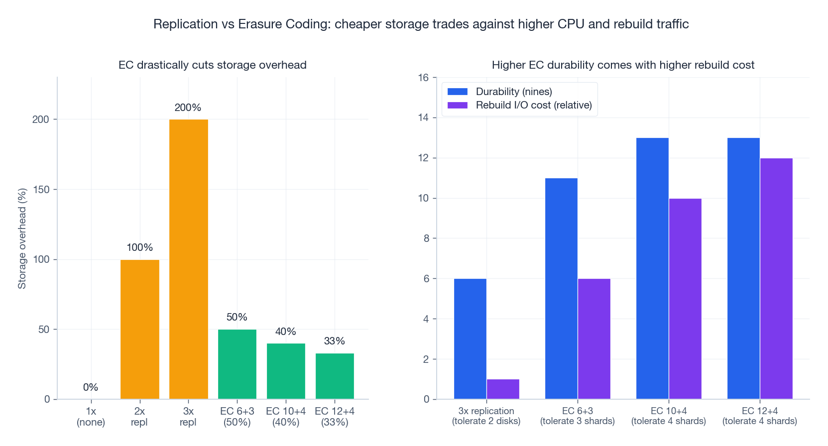
With k+m Reed-Solomon erasure coding, each object is split into k data shards plus m parity shards. The object survives any m shard losses; the storage overhead is m/k.
| Scheme | Overhead | Failures tolerated | Read amplification on rebuild |
|---|---|---|---|
| 3x replication | 200% | 2 disks | 1 (one extra read) |
| EC 6+3 | 50% | 3 shards | 6 (must read 6 shards to reconstruct) |
| EC 10+4 | 40% | 4 shards | 10 |
| EC 12+4 | 33% | 4 shards | 12 |
The trade-off is brutal but predictable:
- Replication: cheap CPU, expensive disks, fast rebuild (just copy one block).
- Erasure coding: cheap disks, expensive CPU + network on rebuild, slower rebuild.
Hot data wants the replication profile (a single read is one HTTP fetch). Cold data wants the EC profile (you rarely touch it, so rebuild cost amortises across years).
11-nines durability is a budget#
S3 advertises “eleven nines” (99.999999999%) of object durability. That is one expected loss per 100 billion object-years. The number is not magic — it is engineered:
- Disk AFR ~1%.
- Spread
k+mshards across at least 3 AZs. - Continuous background scrubbing detects bit-rot before it overlaps with a disk failure.
- Repair is bandwidth-throttled but always running.
The practical lesson: durability is not “we have 3 copies”, it is “we can repair a copy faster than the next failure arrives”. If you build your own storage, instrument the repair pipeline first.
Distributed file systems: HDFS and Ceph#
When you do need POSIX-ish semantics across many machines, two reference designs dominate: HDFS (master-coordinated, append-mostly) and Ceph (peer-to-peer, fully featured).
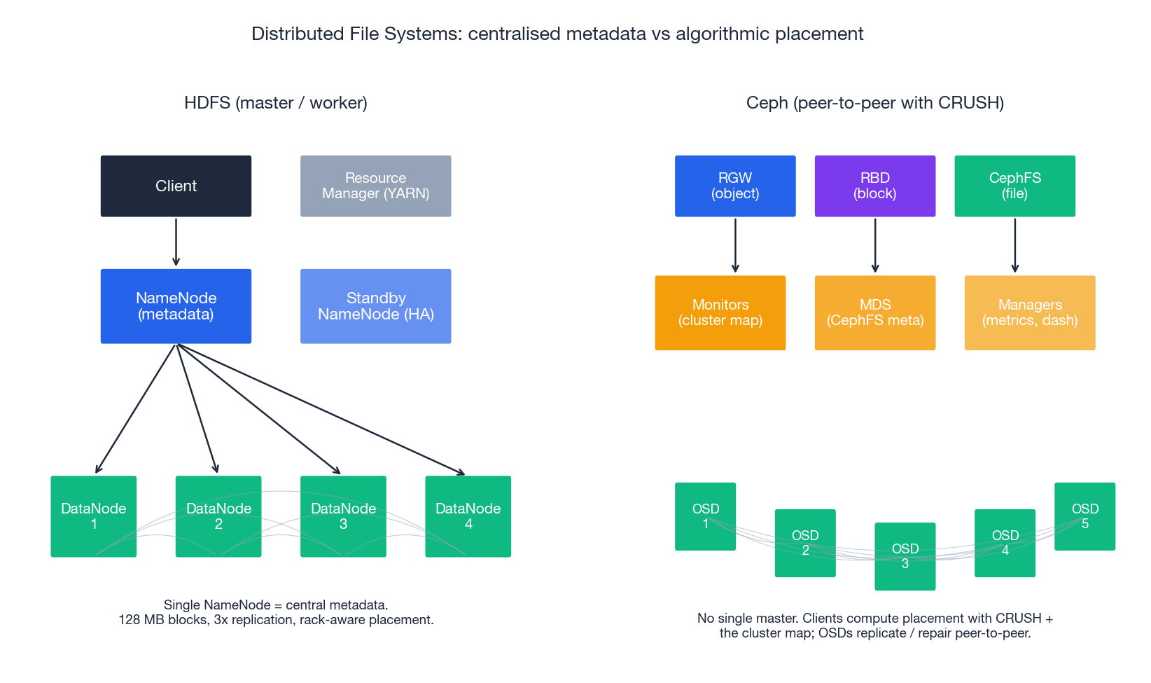
HDFS — master-coordinated, batch-tuned#
HDFS is built on three opinions:
- Files are large, written once, and read many times (logs, parquet, video). The block size default is 128 MB for exactly this reason.
- Failure is normal; replicate at the block level, never at the file level.
- Move computation to the data (the data-locality principle MapReduce was built on).
Architecture:
- NameNode — single source of truth for the namespace and block locations. The active NameNode is paired with a Standby NameNode sharing edits via a JournalNode quorum (Quorum Journal Manager) for HA.
- DataNodes — store the blocks. Default replication factor 3.
- Block placement — first replica on the writer’s node (or a random one if the writer is outside the cluster), second on a different rack, third on another node in the same rack as the second. This survives a full-rack outage while keeping rack-local reads fast.
| |
| |
HDFS is the wrong tool for: small files (each consumes ~150 bytes of NameNode RAM), random writes (it is append-only), or low-latency lookups. For everything else in the Hadoop / Spark ecosystem, it is still excellent.
Ceph — one cluster, three interfaces#
Ceph’s contribution is unified storage: a single RADOS cluster exposing block (RBD), object (RGW), and file (CephFS) interfaces, all backed by the same OSDs.
Two ideas make Ceph different from HDFS:
- No central metadata server for placement. Placement is computed by CRUSH (Controlled Replication Under Scalable Hashing), a pseudo-random algorithm that takes the object name and the cluster map and emits a deterministic OSD set. This eliminates the NameNode bottleneck.
- Self-managing OSDs. Each OSD knows its peers and runs replication, scrubbing, and recovery without a central scheduler.
| |
| |
| |
The price of Ceph’s flexibility is operational weight: tuning CRUSH rules, balancing PGs, capacity planning OSDs, and monitoring rebuild traffic are full-time activities at scale. Most teams should start with the cloud’s managed object/block service and reach for Ceph only when a hard requirement (data sovereignty, on-prem footprint, custom hardware) forces the issue.
Replication strategy and operations#
Synchronous vs asynchronous replication#
| Aspect | Synchronous | Asynchronous |
|---|---|---|
| Consistency | Strong (write returns only after all replicas ack) | Eventual |
| Latency | RTT-bound by the slowest replica | Local disk only |
| RPO | 0 | seconds - minutes |
| Throughput | Limited by slowest link | Limited by primary disk |
| When to use | Financial ledgers, primary database HA in one region | Cross-region DR, analytics replicas |
A common pattern: synchronous within a region (across AZs, sub-millisecond) plus asynchronous across regions (DR replica with a few-second RPO).
Quorum#
For N replicas and read/write quorums R and W:
W + R > Nguarantees a read overlaps with the latest write.W = Nis the strongest writes (no progress on any failure);W = 1is the weakest.- Dynamo-style stores let the application choose
RandWper request; ZooKeeper/etcd hard-codeW = R = majority.
Lifecycle policies — automate the cost story#
Most cost optimisation is a few lines of policy, not engineering work. Move logs to IA at 30 days, Glacier at 90, delete at 365; expire incomplete multipart uploads; transition object versions:
| |
Backup, RTO and RPO#
| Strategy | RTO | RPO | Cost | Use case |
|---|---|---|---|---|
| Hot standby (multi-region active-active) | seconds | ~zero | 2-3x | payments, social feeds |
| Warm standby (replica idle, scaled up on failover) | minutes | seconds | 1.2-1.5x | most production web apps |
| Pilot light (data replicated, infra absent) | hours | minutes | 1.05-1.1x | internal apps |
| Backup-restore only | hours - days | hours | 1.01x | dev / analytics |
The right answer is rarely the strictest one — it is the one whose cost matches the business loss per minute of downtime.
Performance optimisation#
Latency tail dominates#
The number to watch is P99 latency, not the average. In a system that fans out to 10 backends and waits for all, the P99 of the request is roughly the P99 of one backend (Dean & Barroso, The Tail at Scale, 2013). Every dependency is a multiplier.
The four levers#
- Parallelism — multipart uploads, range GETs, concurrent prefixes.
- Locality — co-locate compute and storage (data-locality in HDFS, AZ-affinity in S3 cross-region setups).
- Caching — LRU at the application, CloudFront in front of public S3, OSS CDN for hot prefixes.
- Compression — zstd is the modern default (level 3 ≈ gzip-6 speed at gzip-9 ratio); use Snappy when CPU is scarce.
A throughput rule of thumb#
A single TCP stream on a long-haul link is bandwidth-limited by window / RTT. A 64 KB default window on a 100 ms RTT path tops out at ~5 Mbit/s. To use a 10 Gbit/s pipe you need either a much larger window (kernel auto-tuning helps) or many concurrent streams. Multipart uploads are the explicit form of “many streams”; this is why they are fast, not just that they are.
Cost engineering#
The three line items#
| Bill component | Driver | Lever |
|---|---|---|
| Storage | GB-month | tiering, compression, dedup, expiration |
| Requests | PUT / GET / LIST count | batching, multipart, prefix design |
| Egress | GB out of region / out of cloud | CDN, in-region compute, peering |
For most teams, egress is the surprise on the bill. A 1 PB cross-region copy at $0.02/GB is $ 20,000. Use intra-region replication where possible; if you must move data out, schedule it through a cheaper transfer family (Direct Connect, dedicated peering, Aliyun’s Cloud Enterprise Network).
A worked cost calculation#
A 1 TB dataset accessed twice a day, stored for 1 year:
- Standard: 1 TB × $0.023 × 12 = **$ 276/yr**, plus negligible request cost.
- Standard + 30-day lifecycle to IA: ~$160/yr storage + IA retrieval costs (~$ 10) ≈ $170/yr.
- Lifecycle to Deep Archive after 90 days, with 2 retrievals/year for re-training: ~$15/yr storage + ~$ 40 retrieval fees ≈ $55/yr.
The point is not the exact numbers — list pricing changes — but the order of magnitude. Lifecycle is a 5-10x cost lever and costs nothing to enable.
FAQ#
Q: HDFS or S3 for a new data lake?
S3 (or its equivalent) for almost any greenfield. Modern engines (Trino, Spark, Flink, DuckDB) read object stores natively, you get separation of storage and compute (scale them independently), and you avoid running a NameNode HA cluster. Use HDFS only when an on-prem footprint or extreme data-locality requirement forces the issue.
Q: When is Ceph worth the operational cost?
Three situations: regulatory requirement to keep data on owned hardware; high-volume block + object workload that would be expensive on a managed cloud; an existing OpenStack environment that benefits from Ceph’s tight integration. For everyone else, the cloud’s managed services are cheaper end-to-end once you account for SREs.
Q: 3 replicas or erasure coding?
Replication for hot, latency-sensitive data; erasure coding for cold data and large objects. Many systems do both automatically (S3 internally, Ceph via tiering pools). The decision rarely needs to be made by the application.
Q: How do I size a cache in front of object storage?
Plot access frequency vs object count and look for the “knee”. A typical web workload caches the top 1-5% of objects to absorb 80-95% of GETs. Beyond that you are paying RAM for diminishing returns. CloudFront / OSS CDN turns this into a configuration choice, not a capacity decision.
Cloud Computing 8 parts
- 01 Cloud Computing (1): Fundamentals and Architecture
- 02 Cloud Computing (2): Virtualization Technology Deep Dive
- 03 Cloud Computing (3): Cloud-Native and Container Technologies
- 04 Cloud Computing (4): Cloud Storage Systems and Distributed Architecture you are here
- 05 Cloud Computing (5): Cloud Network Architecture and SDN
- 06 Cloud Computing (6): Cloud Security and Privacy Protection
- 07 Cloud Computing (7): Cloud Operations and DevOps Practices
- 08 Cloud Computing (8): Multi-Cloud and Hybrid Architecture