
Kernel Methods (5): Kernel SVM, Kernel PCA, and Kernel Ridge Regression
The classic algorithms, kernelized — SVM's dual form, Kernel PCA's eigendecomposition in feature space, and Kernel Ridge's closed-form solution. With sklearn code and worked examples.
Your features are two-dimensional, your data is clearly a circle inside a circle, and LinearSVC is at 50% accuracy with the wide-eyed look of an algorithm that genuinely believes a straight line is the answer. You stare at the scatter plot, you stare at the model, and somewhere in the back of your head the words kernel SVM surface. You type kernel='rbf', the accuracy jumps to 0.98, and the rest of the afternoon you wonder what exactly just happened — and why the same trick also gives you a Kernel PCA that unfolds a Swiss roll and a Kernel Ridge regressor that fits a sine wave with three lines of code.

The previous four parts built the machinery: why linear methods fail (Part 1 ), what a positive-definite kernel is (Part 2 ), why the RKHS makes the lifted space behave like a Hilbert space (Part 3 ), and which kernels you’d actually pick off the shelf (Part 4 ). This part is the payoff. We take three textbook linear algorithms — soft-margin SVM, PCA, ridge regression — and watch them kernelize in three nearly identical moves. Each one ends up with the same shape of solution, an $n$ -by-$n$ Gram matrix where a $d$ -by-$d$ covariance used to be, and an answer expressible purely in inner products. That is not a coincidence; it is the representer theorem, and by the end of this post you should feel it.
You will leave with three deliverables. First, the SVM dual derived end to end, with every Lagrangian step justified and the KKT regimes labelled. Second, Kernel PCA as the eigendecomposition of a centred Gram matrix, with the centring formula nobody bothers to derive but everybody secretly looks up. Third, the kernel ridge closed-form solution and its exact equivalence to Gaussian process regression. The pattern is identical in all three: write the loss, invoke the representer theorem, replace inner products with kernel evaluations, solve a finite linear-algebra problem. Three algorithms, one move.
Kernel SVM: from primal to dual#
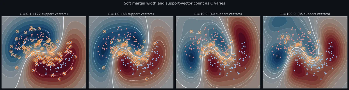
$$\min_{w, b, \xi}\ \tfrac{1}{2}\|w\|^2 + C\sum_{i=1}^n \xi_i \quad \text{s.t.}\quad y_i\bigl(\langle w, x_i\rangle + b\bigr) \geq 1 - \xi_i,\ \ \xi_i \geq 0.$$Two parameters do all the work. The norm $\|w\|$ controls the margin width — small $\|w\|$ is a wide margin. The constant $C$ controls how much slack the model is allowed to buy — small $C$ tolerates many violators and gives a fat, smooth margin; large $C$ forces the boundary to bend around every difficult point.
In the primal, the data lives inside $w$ as raw coordinates $x_i \in \mathbb{R}^d.$ If $d$ is small, fine. If $d$ is millions, or — worse — infinite because we want a kernel, the variable $w$ is unusable. The kernel trick is exactly the rewrite that lets us throw $w$ away. We never store the weight vector, never even define it; we work entirely with $n$ dual coefficients $\alpha_i$ on the $n$ training points. The dimensionality of the input space drops out of the cost. That is what makes kernels tractable and what makes the dual the canonical SVM formulation.
A second observation worth making before we dive in: the primal is convex. The objective $\tfrac{1}{2}\|w\|^2 + C\sum_i \xi_i$ is convex and quadratic in $w$ and linear in $\xi,$ and the constraints are affine. Strong duality holds, the KKT conditions are both necessary and sufficient, and there is exactly one global optimum. None of this is true for neural networks, and it is the reason SVMs survive as a respected baseline even in 2026 — when they work, you know they work, with no doubt about local minima or initialisation.
$$\mathcal{L}(w, b, \xi, \alpha, \mu) = \tfrac{1}{2}\|w\|^2 + C\sum_i \xi_i - \sum_i \alpha_i \bigl[y_i(\langle w, x_i\rangle + b) - 1 + \xi_i\bigr] - \sum_i \mu_i \xi_i.$$ $$\frac{\partial \mathcal{L}}{\partial w} = 0 \implies w = \sum_i \alpha_i y_i x_i,$$ $$\frac{\partial \mathcal{L}}{\partial b} = 0 \implies \sum_i \alpha_i y_i = 0,$$ $$\frac{\partial \mathcal{L}}{\partial \xi_i} = 0 \implies \alpha_i + \mu_i = C.$$The first equation is the one to stare at. It says the optimal weight vector is a linear combination of training points, weighted by $\alpha_i y_i.$ This is the representer theorem appearing organically out of the SVM derivation, before we’ve even mentioned kernels. We did not assume it; we derived it. And once we have it, the rest of the machinery falls into place automatically.
$$\max_{\alpha}\ \sum_i \alpha_i - \tfrac{1}{2}\sum_{i, j} \alpha_i \alpha_j y_i y_j \langle x_i, x_j\rangle \quad \text{s.t.}\quad 0 \leq \alpha_i \leq C,\ \sum_i \alpha_i y_i = 0.$$The data appears only through the inner product $\langle x_i, x_j\rangle.$ Replace every such inner product with $K(x_i, x_j),$ and the optimisation problem has not changed shape — same $n$ variables, same constraints, same quadratic programming solver. The non-linearity is hidden inside $K.$ That is the kernelized dual.
$$f(x) = \sum_{i \in \text{SV}} \alpha_i y_i K(x_i, x) + b,$$where the sum is restricted to support vectors — the points with $\alpha_i > 0.$ By complementary slackness from the KKT conditions, only the points that sit on or inside the margin have non-zero $\alpha,$ and the rest are sparse zeros. A typical RBF SVM on a clean dataset keeps maybe 5–20% of the training points as support vectors. That sparsity is the practical reason SVMs scale at all in the kernelized regime: prediction cost depends on $n_{\text{SV}},$ not on $n.$
KKT in one breath. The Karush–Kuhn–Tucker conditions for this problem partition the training points into three regimes:
- $\alpha_i = 0:$ point is outside the margin, on the right side of the boundary. Ignored.
- $0 < \alpha_i < C:$ point is exactly on the margin. $\xi_i = 0.$ On-margin support vector.
- $\alpha_i = C:$ point has $\xi_i > 0$ — it’s inside the margin or misclassified. Margin-violating support vector.
The threshold $C$ acts as an upper cap on how much influence any single point is allowed to have. That cap is the entire reason soft-margin SVM is robust to outliers in a way that hard-margin SVM is not: a single label-noise point can never command more than $C$ worth of decision boundary. Hard-margin SVM (which corresponds to $C = \infty$ ) lets one outlier ruin everything; soft-margin SVM gracefully absorbs it.
$$b = y_i - \sum_{j \in \text{SV}} \alpha_j y_j K(x_j, x_i).$$In practice, you compute $b$ for every on-margin support vector and average, which gives a numerically stable estimate. If there are no on-margin support vectors (rare but possible at high $C$ ), you use the standard trick of averaging over all SVs with a fix-up.

Kernel SVM in practice#
The dual gives you the theory; sklearn gives you a one-liner. The kernel SVM workhorse is sklearn.svm.SVC, and 90% of the tuning effort goes into two knobs.
| |
The $C$ knob. As covered above, $C$ is the cost of slack. The geometric interpretation is more useful than the algebraic one. Small $C$ widens the margin until many training points are inside it — the boundary looks blurry, almost like a logistic regression fit, and it generalises well because individual points have little leverage. Large $C$ shrinks the margin until almost no points are inside — the boundary squirms around every difficult example, and you start overfitting label noise. A good default is $C=1;$ start there and double in either direction. If you find yourself wanting $C > 100,$ stop and ask whether you really want a soft-margin SVM or whether you should be looking at a different algorithm entirely.
$$\gamma_0 = \frac{1}{2 \cdot \mathrm{median}(\|x_i - x_j\|^2)}.$$Then log-grid one decade either way. If the optimum lands at the edge of your grid, you grid-searched too narrowly; extend.
The interaction. $C$ and $\gamma$ are not independent. A small $\gamma$ (smooth kernel) tolerates a larger $C$ before overfitting, because each support vector’s vote is spread out. A large $\gamma$ (sharp kernel) needs a small $C$ to compensate, otherwise the model concentrates all decision weight on the noisiest points. When you grid-search, you’ll typically see a ridge in the validation surface where good $(C, \gamma)$ pairs lie roughly along a diagonal — small $\gamma$ with large $C$ on one end, large $\gamma$ with small $C$ on the other. That ridge is the model’s effective complexity contour, and grid search is really just locating it. Two-dimensional grid search is sufficient for most use cases; Bayesian optimisation buys you very little for only two hyperparameters.
A common mistake. People standardise their features for LogisticRegression but forget to do it for SVC. The RBF kernel computes $\|x - y\|^2$
in raw feature space — if one feature has range $[0, 1]$
and another $[0, 10^6],$
the second one swamps the kernel and the first might as well not exist. Always standardise (StandardScaler) before fitting any kernel SVM. The median heuristic also assumes standardised features when you compute $\gamma_0;$
on raw features it returns a useless value. The same warning applies to any distance-based or kernel-based method — KNN, k-means, Gaussian processes — but SVM is where it most often bites the unwary, because SVMs look like such a “high-tech” algorithm that people forget the kernel sees only raw coordinates.
Multiclass. SVMs are intrinsically binary. sklearn’s SVC handles multiclass via one-vs-one decomposition (default) — for $K$
classes, it trains $\binom{K}{2}$
binary SVMs. This is more expensive than one-vs-rest for large $K,$
but in practice $K$
is rarely large enough for it to matter, and the one-vs-one classifier is usually more accurate. If you have $K > 20,$
consider switching to logistic regression with multinomial softmax, or to a tree-based ensemble.
Probability outputs. SVMs do not natively produce probabilities. sklearn’s SVC(probability=True) fits a Platt-scaled logistic regression on top of the SVM scores, which costs an extra round of cross-validation at training time and produces probabilities that are usually well-calibrated but slightly worse than the raw classifier accuracy. If you need probabilities, you may as well use logistic regression directly; the SVM advantage was always the geometric margin, not the probabilistic interpretation.
Computational reality. The training cost of kernel SVM is roughly $\mathcal{O}(n^2)$ to $\mathcal{O}(n^3)$ in the number of training points — building the Gram matrix is $\mathcal{O}(n^2 d)$ and solving the QP is between quadratic and cubic depending on the solver. Prediction cost is $\mathcal{O}(n_{\text{SV}} \cdot d)$ per query. This is why kernel SVMs are wonderful at $n = 10^3,$ tolerable at $n = 10^4,$ and infeasible at $n = 10^6.$ Part 7 will cover the approximations — Nyström, random Fourier features, SGD-based linearisation — that push that ceiling.
Kernel PCA: eigendecomposition in feature space#
PCA in its textbook form takes a centred data matrix $X \in \mathbb{R}^{n \times d}$ and eigendecomposes the $d \times d$ covariance matrix $C = \tfrac{1}{n} X^\top X.$ The top $k$ eigenvectors are the principal directions, and projecting any new point onto them gives a $k$ -dimensional code. The whole point of standard PCA is that those directions are linear in the input space — which is sometimes great (when your data really does live near a linear subspace) and sometimes catastrophic (when it lives on a curled manifold).
Kernel PCA replaces “eigendecompose the $d \times d$ covariance” with “eigendecompose the $n \times n$ centred Gram matrix.” The result is the principal components of the feature map $\phi(X),$ even though we never write $\phi$ down. This is the same trick as SVM — replace the explicit feature representation with inner products and an $n \times n$ matrix — applied to an unsupervised problem.
$$C_\phi = \frac{1}{n}\sum_i \phi(x_i) \phi(x_i)^\top,$$ $$v_k = \sum_i \alpha_i^{(k)} \phi(x_i).$$ $$K \alpha^{(k)} = n \lambda_k \alpha^{(k)},$$where $K$ is the $n \times n$ Gram matrix with entries $K_{ij} = \langle \phi(x_i), \phi(x_j)\rangle = K(x_i, x_j).$ The eigenproblem on the infinite-dimensional covariance operator has reduced to an eigenproblem on a finite Gram matrix. That’s the whole content of Kernel PCA.
$$\tilde{K} = K - \mathbf{1}_n K - K \mathbf{1}_n + \mathbf{1}_n K \mathbf{1}_n,$$where $\mathbf{1}_n$ is the $n \times n$ matrix of $1/n$ ’s. This formula is one of the few things in kernel methods that you should just memorise — every kernel PCA implementation does this step, and getting the signs wrong gives you garbage components. Derivation: expand $\tilde{K}_{ij} = \langle \tilde{\phi}(x_i), \tilde{\phi}(x_j)\rangle$ using bilinearity and the definition of $\tilde{\phi},$ and the four terms drop out.
Normalisation. The eigenvectors $\alpha^{(k)}$
that come out of eig(K) are unit-norm in $\mathbb{R}^n,$
but the corresponding $v_k = \sum_i \alpha_i^{(k)} \phi(x_i)$
is generally not unit-norm in $\mathcal{H}_K.$
Imposing $\|v_k\|^2 = \alpha^{(k)\top} K \alpha^{(k)} = 1$
gives the rescaling $\alpha^{(k)} \to \alpha^{(k)} / \sqrt{n \lambda_k}.$
sklearn’s KernelPCA does this for you, but if you ever roll your own you must remember it; without the rescaling the projection coordinates have the wrong scale.
Note the asymmetry with linear PCA: here the projection coefficients $\alpha_i^{(k)}$ are weights on the training points, not directions in input space. You cannot reconstruct $x$ from $z_k(x)$ without solving a pre-image problem, which is one of Kernel PCA’s biggest limitations and the topic of an entire small literature (see Mika et al., 1998). For visualisation purposes the pre-image is usually not needed, but for any task that needs to map back to input space (denoising, generation) it is the dominant difficulty.
Why it works on non-linear manifolds. If your data is a Swiss roll embedded in 3D, the data lives on a 2-dimensional manifold that linear PCA can’t see — the principal directions of the rolled-up sheet point in the “wrong” directions because PCA only knows about straight lines. Kernel PCA with an RBF kernel computes the principal components of $\phi(X),$ where $\phi$ implicitly maps every point to its similarity profile against the training set. In that representation, the manifold is “unrolled,” and the top eigenvectors correctly recover the two intrinsic dimensions of the roll. This is closely related to spectral embedding methods like Isomap and Laplacian eigenmaps, all of which can be viewed as Kernel PCA with a particular data-dependent kernel.

Kernel PCA in practice#
The sklearn API is sklearn.decomposition.KernelPCA, and it’s a near-drop-in replacement for PCA:
| |
Choosing $\gamma$ . As with kernel SVM, $\gamma$ controls bandwidth and is the single most important hyperparameter. Unlike SVM, there is no labelled signal to grid-search against — Kernel PCA is unsupervised. Three practical strategies:
- Median heuristic. Compute $\gamma_0$ from pairwise distances, then visually inspect a few decades around it. For dimensionality reduction with a downstream task, you can grid-search $\gamma$ using the downstream task’s performance as the signal.
- Reconstruction error. Project to $k$
components, then reconstruct using
KernelPCA(fit_inverse_transform=True), and pick $\gamma$ that minimises the mean reconstruction error on a hold-out set. This is principled but limited because the reconstruction itself depends on $\gamma$ and the kernel. - Downstream classifier accuracy. If Kernel PCA is a preprocessing step for an SVM or random forest, $\gamma$ is just another hyperparameter and you fold it into the same cross-validation as the classifier’s.
When it pays off. Kernel PCA is most useful when (a) you have non-linearly structured data, (b) you want to visualise the structure in 2D or 3D, and (c) the structure is best characterised by smooth, local similarity. Swiss roll, S-curve, moons, and concentric circles are the canonical “Kernel PCA shines” datasets. On high-dimensional, sparse, or already-linear data, standard PCA is almost always equal or better — and much cheaper, since standard PCA scales as $\mathcal{O}(d^2 n + d^3)$ while kernel PCA is $\mathcal{O}(n^3).$
When it fails. Kernel PCA is fragile in two specific ways. First, on noisy data, the top eigenvectors of the Gram matrix can be dominated by noise patterns rather than signal — small $\gamma$ helps but blurs the structure. Second, on data with multiple disconnected manifolds (e.g. two well-separated blobs each with their own curvature), the top components often capture the between-cluster variation rather than the within-cluster structure, which may or may not be what you want. If you specifically want within-cluster structure, you might be better off with t-SNE or UMAP, which optimise a local-neighbourhood-preserving loss instead of a variance-maximising one.

Computational note. The $\mathcal{O}(n^3)$
cost of eigendecomposing the Gram matrix is the binding constraint. For $n > 5000,$
use the eigen_solver='arpack' option to compute only the top $k$
eigenvectors, which drops the cost to roughly $\mathcal{O}(n^2 k).$
For very large $n,$
you’ll want the Nyström approximation, which we’ll meet in Part 7
.
vs. t-SNE and UMAP. Modern practice often reaches for t-SNE or UMAP rather than Kernel PCA for non-linear visualisation. The reasons are: (i) t-SNE/UMAP explicitly optimise for preserving local neighbourhoods, which is what your eye cares about in a 2D plot; (ii) they handle large $n$ much better in practice (UMAP scales near-linearly); (iii) they don’t require the user to pick a kernel. Kernel PCA’s advantages over t-SNE/UMAP are: (i) it has a closed-form, deterministic projection function for new test points (t-SNE doesn’t, UMAP does but only approximately); (ii) it is faithful to the variance structure rather than the neighbourhood structure, which is what you want if downstream you’re going to feed it into a linear classifier; (iii) it has a single hyperparameter, not three. For exploratory visualisation, use UMAP. For a preprocessing step before a downstream model, use Kernel PCA.
Kernel ridge regression: the closed-form elegance#
$$\min_w\ \tfrac{1}{2}\|y - Xw\|^2 + \tfrac{\lambda}{2}\|w\|^2,$$ $$\hat{w} = (X^\top X + \lambda I)^{-1} X^\top y.$$The $\lambda$ term regularises the inverse and keeps things numerically stable even when $X^\top X$ is rank-deficient. The closed-form is the reason ridge is everyone’s go-to regression baseline: no optimisation loop, no hyperparameter beyond $\lambda,$ trivially differentiable, well-conditioned.
$$\hat{f}(x) = \langle w, \phi(x)\rangle = \sum_i \alpha_i \langle \phi(x_i), \phi(x)\rangle = \sum_i \alpha_i K(x_i, x).$$ $$\min_\alpha\ \tfrac{1}{2}\|y - K\alpha\|^2 + \tfrac{\lambda}{2} \alpha^\top K \alpha.$$ $$\alpha = (K + \lambda I)^{-1} y.$$ $$\hat{f}(x) = \mathbf{k}(x)^\top \alpha = \mathbf{k}(x)^\top (K + \lambda I)^{-1} y,$$where $\mathbf{k}(x) \in \mathbb{R}^n$ has entries $\mathbf{k}(x)_i = K(x_i, x).$ Compare to the linear ridge formula $\hat{f}(x) = x^\top (X^\top X + \lambda I)^{-1} X^\top y;$ the structure is identical, with $K$ replacing $X^\top X$ and $\mathbf{k}(x)$ replacing $X^\top x.$ This is the kernel trick at its purest — replace each matrix with its kernelised analogue, and the algorithm goes through without further modification.
No iteration. Unlike SVM, there is no QP to solve. The whole training is a single linear solve. For $n$ training points and a kernel with $\mathcal{O}(d)$ evaluation cost, the total complexity is $\mathcal{O}(n^2 d)$ to build the Gram matrix plus $\mathcal{O}(n^3)$ to invert it. Prediction is $\mathcal{O}(n d)$ per query, which is the cost of evaluating the kernel against every training point. There is no sparsity — every $\alpha_i$ is generically non-zero. This is the price of having a closed form: you trade away SVM’s sparse-support-vector structure in exchange for not having to solve a QP.
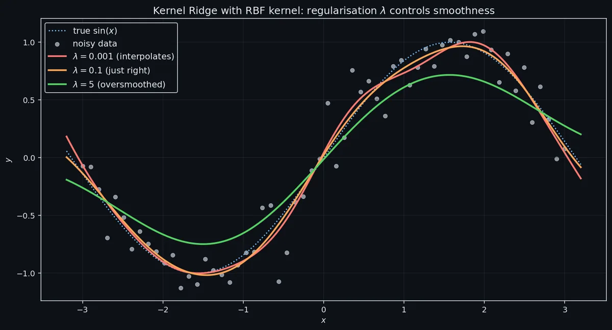
The role of $\lambda.$ $\lambda$ is the only knob besides the kernel’s own hyperparameters. Small $\lambda$ means the model interpolates the training data — at $\lambda = 0$ the prediction at any training point $x_i$ is exactly $y_i,$ which is great until your training labels are noisy. Large $\lambda$ shrinks all $\alpha_i$ towards zero, the predictions regress towards the mean, and the model underfits. Use cross-validation; log-grid $\lambda \in \{10^{-6}, \ldots, 10^{2}\}$ and pick by held-out MSE. Leave-one-out cross-validation for kernel ridge is especially cheap because it can be computed from a single fit using a closed-form trick (the LOO residuals factor through the diagonal of the hat matrix $H = K(K + \lambda I)^{-1}$ ).
| |
Note that sklearn calls the regularisation parameter alpha (matching standard ridge) rather than $\lambda;$
they are the same thing. The kernel and gamma arguments behave exactly as in SVC. Kernel ridge does not have a $C$
parameter because it does not have a hinge loss — the entire loss is squared error, and $\lambda$
alone controls regularisation.
A practical note on conditioning. The matrix $K + \lambda I$
can become numerically singular if $\lambda$
is very small and the kernel is very sharp (large $\gamma$
) and you have nearly duplicate training points. The symptom is a LinAlgError or wildly oscillating predictions. The fixes are: increase $\lambda,$
standardise features, deduplicate training points, or switch to a numerically stable solver (Cholesky decomposition of $K + \lambda I,$
which sklearn does internally). The Cholesky factorisation works because $K + \lambda I$
is positive definite by construction whenever $K$
is positive semi-definite and $\lambda > 0;$
if it ever fails to be positive definite, your kernel is misimplemented.
Kernel ridge vs Gaussian processes#
$$\hat{f}_{\text{KRR}}(x) = \mathbf{k}(x)^\top (K + \lambda I)^{-1} y = \mathbb{E}\bigl[f(x) \mid \mathcal{D}\bigr]_{\text{GP}}.$$This is not a metaphor or an “if you squint” similarity — they are the same formula. So why are they treated as two different algorithms?
The probabilistic interpretation is what differs. GP regression doesn’t just give you a mean prediction; it gives you a full posterior distribution with a variance at every test point. Kernel ridge gives you only the point estimate. That extra variance is the entire reason GPs are popular in Bayesian optimisation, active learning, and uncertainty quantification — you know how much you don’t know at any query point, and the variance grows in regions of input space without nearby training data. Kernel ridge has none of that.
The cost is the same. Both algorithms require the same $\mathcal{O}(n^3)$ inverse, so there is no computational reason to pick one over the other. Use kernel ridge when you only need point predictions; use GP when you need calibrated uncertainty. We will cover the GP side of this duality in detail in Part 6 , including how the GP framework lets you learn the kernel hyperparameters by maximising marginal likelihood — a luxury that kernel ridge regression does not have.
A subtle equivalence. The kernel ridge hyperparameter $\lambda$ corresponds to the GP’s noise variance $\sigma_n^2.$ The kernel’s bandwidth $\gamma$ corresponds to the GP’s length scale. The GP framework gives you a principled way to learn these from the data (maximum marginal likelihood) rather than cross-validating them, which is one of the practical advantages of the Bayesian framing. Cross-validation for kernel ridge requires picking a CV scheme, a metric, and a grid; marginal likelihood for GPs has none of those choices to make. The trade-off is that marginal likelihood can overfit in low-data regimes, whereas held-out CV cannot.
The unified view: representer theorem strikes thrice#
Step back and notice the shape of all three derivations. In SVM, $w = \sum_i \alpha_i y_i \phi(x_i).$ In Kernel PCA, the principal direction $v_k = \sum_i \alpha_i^{(k)} \phi(x_i).$ In Kernel Ridge, $w = \sum_i \alpha_i \phi(x_i).$ Each algorithm’s optimal solution is a linear combination of the training points in feature space, weighted by $n$ coefficients. The infinite-dimensional optimisation collapses to an $n$ -dimensional one, and the only object that ever appears is the Gram matrix $K.$
This is no coincidence. It is the representer theorem, which we proved in Part 3 and which says: for any loss function that depends on $f$ only through its values at the training points $\{f(x_i)\}_{i=1}^n,$ plus a monotonically increasing function of $\|f\|_{\mathcal{H}_K},$ the optimal $f^*$ in the entire RKHS lies in the finite-dimensional subspace spanned by $\{K(x_i, \cdot)\}_{i=1}^n.$ SVM, PCA, and ridge all fit this template, and so do logistic regression, Fisher discriminant, quantile regression, and any number of other classical algorithms. Once you’ve seen one kernelisation, you’ve seen them all.
Complexity at a glance:
| Algorithm | Training cost | Prediction cost | Sparsity | Output |
|---|---|---|---|---|
| Kernel SVM | $\mathcal{O}(n^2)$ to $\mathcal{O}(n^3)$ | $\mathcal{O}(n_{\text{SV}} d)$ | Yes — only SVs | Class label |
| Kernel PCA | $\mathcal{O}(n^3)$ eigendecomp | $\mathcal{O}(n d)$ per component | No | $k$ -dim code |
| Kernel Ridge | $\mathcal{O}(n^3)$ linear solve | $\mathcal{O}(n d)$ | No | Real prediction |
All three are dominated by an $\mathcal{O}(n^3)$ matrix operation, which is the structural reason kernel methods don’t scale to web-data sizes without the approximations we’ll meet in Part 7 . The differences are in the kind of matrix operation (QP for SVM, eigendecomposition for PCA, linear solve for ridge) and in whether the output is sparse — SVM has sparse $\alpha$ thanks to KKT complementary slackness, while PCA and ridge generically don’t. Memory cost in all three cases is $\mathcal{O}(n^2)$ for the Gram matrix, which becomes the binding constraint around $n = 30{,}000$ on a 16 GB machine using float64.

A meta-observation. Whenever you see a linear algorithm in the wild — Fisher LDA, canonical correlation analysis, partial least squares, kernel logistic regression — and you find yourself thinking “this would be much more powerful if it were non-linear,” check whether the loss depends on the data only through inner products. If yes, the representer theorem applies, the kernelisation is mechanical, and you can probably do it in an afternoon. If no, you need a different trick (often neural-net-style explicit feature learning, which is what Part 8 will compare).
A second meta-observation. Kernels are not the only way to add non-linearity to a linear algorithm. The other paths are: (i) explicit basis expansion (polynomial features, B-splines, Fourier features), which is essentially the explicit version of the kernel trick and recovers it in the limit; (ii) ensembles of linear models on partitions of the input space (decision trees, random forests, gradient boosting); (iii) deep learning, which composes affine layers with element-wise non-linearities to learn the feature map $\phi$ itself rather than fixing it in advance. Each path has a regime where it wins. Kernels win in low-data, smooth-function, calibrated-uncertainty regimes. Trees win on tabular data with categorical features and irregular interactions. Deep learning wins on perceptual data (vision, audio, language) where the feature hierarchy needs to be learned from millions of examples. Part 8 will compare these head-to-head.
What’s next#
Part 6 takes the kernel ridge / GP equivalence and runs with it. We’ll build Gaussian processes properly: the prior over functions, the posterior given data, the choice of mean function, hyperparameter learning by maximum marginal likelihood, and what the posterior variance is actually telling you. By the end of Part 6 you’ll see kernel ridge as one special case of a much richer probabilistic framework, and you’ll be ready to do Bayesian optimisation, active learning, and uncertainty-aware regression in real settings.
This is Part 5 of Kernel Methods (8 parts). Previous: Part 4 — Common Kernel Families · Next: Part 6 — Gaussian Processes
Kernel Methods 8 parts
- 01 Kernel Methods (1): Why We Need Them — Hitting the Ceiling of Linear Algorithms
- 02 Kernel Methods (2): Mathematical Foundations — Positive-Definite Kernels and Mercer's Theorem
- 03 Kernel Methods (3): RKHS — The Theoretical Soul of Kernel Methods
- 04 Kernel Methods (4): Common Kernel Families — RBF, Matern, Polynomial, Periodic, and More
- 05 Kernel Methods (5): Kernel SVM, Kernel PCA, and Kernel Ridge Regression you are here
- 06 Kernel Methods (6): Gaussian Processes — When Kernels Meet Bayesian Inference
- 07 Kernel Methods (7): Large-Scale Kernels — Nystrom Approximation and Random Fourier Features
- 08 Kernel Methods (8): Deep Kernel Learning vs Deep Learning — A Practitioner's Guide


