
Essence of Linear Algebra (12): Sparse Matrices and Compressed Sensing — Less Is More
Sparsity is everywhere: JPEG photos, MRI scans, genomic data. Compressed sensing exploits this to recover signals from far fewer measurements than traditional theory requires. This chapter covers L1 regularization, LASSO, the RIP condition, and recovery algorithms.

The “Less Is More” Miracle#
A raw 24-megapixel photograph weighs in at roughly 70 MB. JPEG compresses it to a few hundred kilobytes — a 100$\times$ reduction — and you cannot tell the difference. A traditional MRI scan takes thirty minutes; a modern compressed sensing MRI gets the same image in five.
Both miracles run on the same engine: sparsity. Most natural signals, written in the right basis, have only a handful of meaningful coefficients. Everything else is essentially zero.
Compressed sensing turns that observation into an algorithm. Because the signal is sparse, you need far fewer measurements than classical sampling theory demands — and you can still reconstruct it exactly. This chapter walks through why.
What you will learn#
- What sparsity means mathematically and why it shows up everywhere
- The$L_0$ /$L_1$ /$L_2$ norms and the geometric reason$L_1$ produces sparse solutions
- LASSO: regression and feature selection in a single optimization
- Compressed sensing theory: the RIP condition, measurement matrices, recovery guarantees
- Algorithms: ISTA, FISTA, Iterative Hard Thresholding, OMP
- Where this is actually used: MRI, single-pixel cameras, genomics, finance
Prerequisites#
- Norms and condition numbers (Chapter 10 )
- Convex optimization (Chapter 11 )
- SVD and low-rank approximation (Chapter 9 )
Sparsity: the Universal Pattern#
Definition#
A vector$\vec{x} \in \mathbb{R}^n$ is $k$ -sparse if at most$k$ of its entries are nonzero:$\|\vec{x}\|_0 \;=\; \bigl|\{\,i : x_i \neq 0\,\}\bigr| \;\leq\; k.$ The$L_0$ “norm” simply counts nonzeros. It is not a real norm — it fails homogeneity ($\|2x\|_0 = \|x\|_0$ ) — but it is the cleanest measure of sparsity we have.
In practice signals are rarely exactly sparse; they are compressible. Sort the coefficients by magnitude and the sorted sequence decays quickly. Truncating to the top$k$ gives a near-perfect approximation. JPEG works exactly this way: compute the DCT, keep the largest few hundred coefficients, throw the rest away.
Sparsity in the wild#
| Domain | Sparse in what basis | Why |
|---|---|---|
| Photos | Wavelets / DCT | Smooth regions have small high-frequency energy |
| Speech | Fourier / Gabor | Voiced sounds concentrate in narrow bands |
| Text (one document) | Vocabulary indicator | A document uses a tiny fraction of all words |
| Social graphs | Adjacency matrix | Each person knows$O(\log n)$ people |
| Genomics | Gene expression | A handful of genes drive any given disease |
| Astronomy | Star-field pixels | Black sky is the rule, stars are the exception |
Sparse representation in a dictionary#
A signal that is dense in the standard basis often becomes sparse after a change of basis. Pick a dictionary$D \in \mathbb{R}^{n \times p}$ whose columns are called atoms, and ask:$\vec{x} \;=\; D\vec{\alpha}, \qquad \vec{\alpha}\;\text{sparse}.$ Common choices:
| Dictionary | Built for | Property |
|---|---|---|
| Fourier basis | Stationary periodic signals | Frequency-domain sparse |
| Wavelet basis | Images, transients | Joint time/scale localization |
| DCT basis | Image blocks (JPEG) | Real-valued Fourier cousin |
| Learned dictionary | Domain-specific data | Fitted from examples (K-SVD) |
When$p > n$ , the dictionary is overcomplete: there are many ways to write$\vec{x}$ , and we hunt for the sparsest one.
Sparse Matrix Storage#
Before diving into recovery, it is worth asking how to store a matrix that is mostly zero. Three formats dominate; they make different trade-offs for build, read, and matrix-vector product.
| Format | What it stores | Strength |
|---|---|---|
| COO | (row, col, value) triples | Easy to construct, easy to convert |
| CSR | data, col_idx, row_ptr | Fast row slicing and$Av$ |
| CSC | data, row_idx, col_ptr | Fast column slicing and$A^\top v$ |
A sparse matrix-vector product costs$O(\text{nnz})$ instead of$O(mn)$ . For a$10^6 \times 10^6$ matrix with one million nonzeros, that is a one-million-times speedup.

The figure shows the same$8 \times 8$
matrix with thirteen nonzeros. COO simply lists each nonzero. CSR compresses the row indices into pointers: indptr[i]:indptr[i+1] is the slice of cols and vals belonging to row$i$
. CSC does the same for columns.
When does this actually save memory? Each nonzero in CSR costs eight bytes for the value plus four bytes for the column index. Storing it as dense costs eight bytes per entry, every entry.

CSR breaks even with dense storage at about 67% density (8 / (8+4)). Below ~10% density — where most real sparse matrices live — the memory and compute savings are an order of magnitude or more.
$L_1$ Regularization: the Practical Key#
$L_0$ is intractable#
Find the sparsest representation of$\vec{x}$ in dictionary$D$ :$\min_{\vec{\alpha}}\;\|\vec{\alpha}\|_0 \quad \text{s.t.}\quad D\vec{\alpha} = \vec{x}.$ This is NP-hard. Naively you would enumerate all$\binom{p}{k}$ possible supports — combinatorial explosion. No polynomial-time algorithm is known for the general problem.
$L_1$ as a convex relaxation#
Replace$\|\cdot\|_0$ with$\|\cdot\|_1 = \sum |\alpha_i|$ :$\min_{\vec{\alpha}}\;\|\vec{\alpha}\|_1 \quad \text{s.t.}\quad D\vec{\alpha} = \vec{x}.$ This problem is a linear program — solvable in polynomial time. The remarkable fact is that, under mild conditions on$D$ , the$L_1$ solution coincides with the$L_0$ solution. Convex relaxation is exact.
Why does$L_1$ promote sparsity? The geometric picture#
Imagine the constraint set$\{\vec{\alpha} : D\vec{\alpha} = \vec{x}\}$ as an affine subspace cutting through$\mathbb{R}^p$ . Minimizing$\|\vec{\alpha}\|_1$ means inflating an$L_1$ ball from the origin until it just kisses the constraint.
- The$L_1$ ball is a diamond: it has sharp corners exactly on the coordinate axes.
- The$L_2$ ball is a sphere: smooth everywhere.
A diamond inflated against a generic line touches it first at a corner — and corners lie on axes, where some coordinates are zero. A sphere touches at a generic surface point with no coordinates forced to zero.

This picture is the entire intuition for why$L_1$ , LASSO, basis pursuit, and compressed sensing exist. Every higher-dimensional version is the same story: the$L_1$ ball in$\mathbb{R}^n$ has$2n$ corners on the axes, and the geometry of “first contact at a corner” persists.
$L_1$ vs $L_2$ at a glance#
| Property | $L_1$ | $L_2$ |
|---|---|---|
| Unit ball | Diamond / cross-polytope | Sphere |
| Solution structure | Many exact zeros (sparse) | All entries small but nonzero |
| Differentiable at zero? | No (subgradient) | Yes |
| Optimization | Proximal / coordinate / LP | Closed form, gradient descent |
| Typical use | Feature selection, CS | Ridge, weight decay |
Elastic Net#
When features are highly correlated, pure$L_1$ tends to pick one feature from a correlated group and drop the rest. Combining the two penalties$\min_{\vec{\beta}}\; \tfrac{1}{2}\|X\vec{\beta} - \vec{y}\|^2 + \lambda_1\|\vec{\beta}\|_1 + \lambda_2\|\vec{\beta}\|_2^2$ keeps the sparsity of$L_1$ while inheriting the stability of$L_2$ . This is the Elastic Net, and in practice it is the safer default for high-dimensional regression.
LASSO Regression#
Definition#
LASSO — Least Absolute Shrinkage and Selection Operator (Tibshirani, 1996):$\min_{\vec{\beta}}\;\tfrac{1}{2}\|X\vec{\beta} - \vec{y}\|^2 \;+\; \lambda\|\vec{\beta}\|_1.$ Two things happen simultaneously: the data term fits$\vec{y}$ , and the$L_1$ penalty drives unimportant coefficients to exactly zero. So LASSO is regression and feature selection in one shot.
Soft thresholding#
For an orthogonal design ($X^\top X = I$ ) the LASSO has a closed-form solution:$\hat\beta_j \;=\; \mathcal{S}_\lambda\!\bigl(\hat\beta_j^{\text{OLS}}\bigr) \;=\; \operatorname{sign}\!\bigl(\hat\beta_j^{\text{OLS}}\bigr)\,\bigl(|\hat\beta_j^{\text{OLS}}| - \lambda\bigr)_+.$ This soft thresholding operator pushes every OLS coefficient toward zero by exactly$\lambda$ , and clamps anything smaller than$\lambda$ to zero outright. Compare with hard thresholding, which leaves large coefficients untouched and zeros the rest — abrupt and unstable.
The LASSO solution path#
Sweep$\lambda$ from$\infty$ down to$0$ :
- Large$\lambda$ : all coefficients are zero.
- Decreasing$\lambda$ : features enter the active set one at a time, each at the$\lambda$ where its correlation with the residual exceeds the threshold. -$\lambda \to 0$ : ordinary least squares.
A beautiful structural fact, due to Efron, Hastie, Johnstone, and Tibshirani (2004): the path is piecewise linear in$\lambda$ . The LARS algorithm exploits this to compute the entire path in roughly the cost of a single OLS fit.
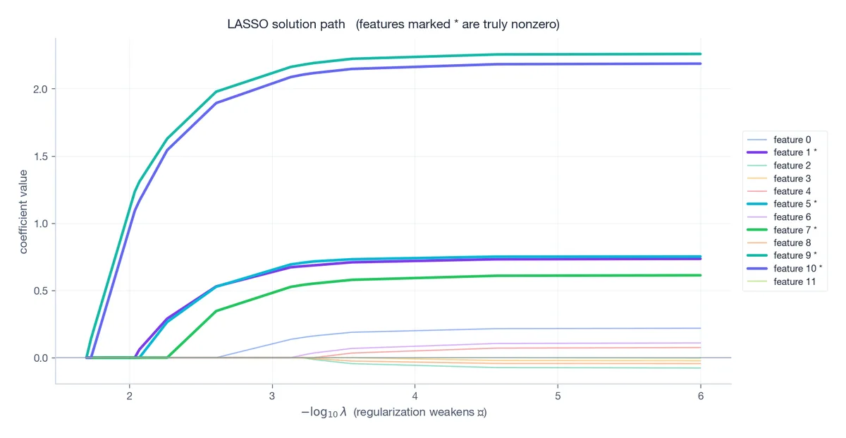
The truly active features (bold) enter early and grow large. Spurious features either never enter or enter late with tiny coefficients. Choose$\lambda$ by cross-validation — usually picking the largest$\lambda$ within one standard error of the minimum-error choice (the “1-SE rule”) to favor parsimony.
Compressed Sensing#

The revolutionary idea#
Shannon-Nyquist says: to recover a band-limited signal you must sample at twice its highest frequency. Period.
Compressed sensing says: if the signal is$k$ -sparse in some basis, you only need$m \;\sim\; k\,\log\!\frac{n}{k}$ linear measurements. For a 256-pixel signal with 10 nonzero wavelet coefficients,$k\log(n/k) \approx 32$ measurements — not 256.
This is not a free lunch; it works because the signal model is much stronger. Shannon-Nyquist asks “any band-limited signal,” compressed sensing asks “any$k$ -sparse signal.” The narrower model permits cheaper sensing.
The measurement model$\vec{y} \;=\; \Phi \vec{x} \;+\; \vec{e},$ with$\vec{x} \in \mathbb{R}^n$ ($k$ -sparse),$\Phi \in \mathbb{R}^{m \times n}$ with$m \ll n$ , and noise$\vec{e}$ . The system$\Phi \vec{x} = \vec{y}$ is underdetermined — infinitely many solutions. Sparsity is the side constraint that selects the right one.#

The figure runs ISTA on random Gaussian$\Phi$ with$m=64$ ,$n=256$ ,$k=10$ . The recovered signal matches the truth to relative error$\sim 10^{-2}$ , with the same support and the same amplitudes. Recall that$k \log(n/k) \approx 32$ – 64 measurements is comfortably above the threshold and recovery is essentially perfect.
The Restricted Isometry Property (RIP)#
When does an underdetermined$\Phi$ preserve enough information to uniquely identify a sparse$\vec{x}$ ? Candès and Tao’s answer is the Restricted Isometry Property.
Definition.$\Phi$ satisfies the$k$ -RIP with constant$\delta_k \in (0,1)$ if$(1 - \delta_k)\|\vec{x}\|_2^2 \;\leq\; \|\Phi\vec{x}\|_2^2 \;\leq\; (1 + \delta_k)\|\vec{x}\|_2^2$ for every$k$ -sparse$\vec{x}$ . In words:$\Phi$ acts almost like an isometry on sparse vectors — it cannot squash two different sparse vectors to (nearly) the same image.

Left: histograms of$\|\Phi\vec{x}\|/\|\vec{x}\|$ over many random$k$ -sparse$\vec{x}$ , for several sparsity levels. The distributions tightly concentrate around 1 — norms are nearly preserved. Right: the empirical worst-case distortion$\delta_k$ as$k$ grows. Beyond some sparsity, the bound$\sqrt{2}-1$ is violated; below it, exact recovery is guaranteed.
The recovery theorem#
Theorem (Candès-Tao, 2005). If$\delta_{2k}(\Phi) < \sqrt{2} - 1 \approx 0.414$ , then every$k$ -sparse$\vec{x}$ is the unique solution of$\min \|\vec{z}\|_1 \quad \text{s.t.}\quad \Phi\vec{z} = \vec{y}, \qquad \vec{y} = \Phi\vec{x}.$ With noise — via Basis Pursuit Denoising,$\min\|\vec{z}\|_1 \,\text{s.t.}\, \|\Phi\vec{z}-\vec{y}\| \leq \epsilon$ – the recovery error is bounded by a constant times$\epsilon$ . Graceful degradation.
Designing$\Phi$ Building deterministic matrices that satisfy RIP for large$k$ is hard. The trick is to flip a coin: random matrices satisfy RIP with overwhelming probability.#
| Construction | $\Phi_{ij}$ | Notes |
|---|---|---|
| Gaussian | $\mathcal{N}(0, 1/m)$ | Universal, easiest to analyse |
| Bernoulli | $\pm 1/\sqrt{m}$ | Cheap arithmetic |
| Partial Fourier | random rows of DFT | Used in MRI, fast transforms |
| Sub-Gaussian | other light-tailed | Same scaling$m \sim k\log(n/k)$ |
Universality — the same$\Phi$ works for any$k$ -sparse signal — is what makes random measurement matrices so practical.
Algorithms#
ISTA — Iterative Shrinkage-Thresholding#
Apply proximal gradient to$\tfrac{1}{2}\|\Phi x - y\|^2 + \lambda\|x\|_1$ :$\boxed{\;\vec{x}^{(t+1)} \;=\; \mathcal{S}_{\lambda/L}\!\left(\vec{x}^{(t)} - \tfrac{1}{L}\Phi^\top\!\bigl(\Phi \vec{x}^{(t)} - \vec{y}\bigr)\right)\;}$ where$L = \|\Phi^\top\Phi\|_2$ is the Lipschitz constant of the smooth part. One gradient step, then a soft threshold. Convergence rate$O(1/t)$ .
| |
FISTA — Nesterov-Accelerated ISTA#
Add a momentum term and the convergence rate jumps from$O(1/t)$ to$O(1/t^2)$ :
| |
IHT — Iterative Hard Thresholding#
If you happen to know the sparsity level$k$ , replace the soft threshold by keep the top-$k$ entries:$\vec{x}^{(t+1)} \;=\; H_k\!\left(\vec{x}^{(t)} - \tfrac{1}{L}\Phi^\top\!\bigl(\Phi \vec{x}^{(t)} - \vec{y}\bigr)\right).$ IHT directly attacks the$L_0$ problem and converges to a$k$ -sparse solution under an RIP-like condition. It is dirt-cheap per iteration: a matrix-vector product plus a partial sort.

The four panels snapshot the iterate at iterations 0, 2, 5, and 30 against the true signal (faint background). After two iterations the support is roughly right; by iteration 30 the amplitudes are dialled in. The residual norm$\|\Phi x_t - y\|_2$ drops by orders of magnitude.
OMP — Orthogonal Matching Pursuit#
A pure greedy algorithm: at each step, pick the atom most correlated with the current residual, add it to the support, and resolve least squares on that support.
| |
OMP is fast and easy to reason about, but greedy: a wrong choice early on cannot be undone. LASSO and FISTA are slower but globally optimal.
Applications#
Compressed sensing MRI#
MRI samples in k-space — the Fourier transform of the image — one row at a time. Sampling all of k-space is what makes MRI slow.
The CS-MRI recipe:
- Acquire a random subset of k-space rows ($m \approx 0.25 n$ is typical).
- Use the fact that MR images are sparse in the wavelet domain.
- Solve$\min \|\Psi \vec{x}\|_1$ s.t.$\Phi \vec{x} \approx \vec{y}$ , where$\Psi$ is the wavelet transform.
Real-world result: 2–8$\times$ shorter scans with equal diagnostic quality. The FDA has cleared multiple CS-MRI products since 2017 (Siemens “Compressed Sensing Cardiac Cine,” GE “HyperSense,” etc.).
Single-pixel camera#
Skip the megapixel sensor entirely. A digital micromirror array projects a sequence of random$\pm 1$ patterns onto the scene; a single photodiode integrates the resulting light into one number per pattern. With$m \sim k \log(n/k)$ patterns you reconstruct an$n$ -pixel image. Indispensable in the infrared and terahertz bands, where pixel arrays are eye-wateringly expensive.
Genomics#
A genomic study has$n \sim 20{,}000$ candidate genes and$m \sim 100$ patients — the classic$n \gg m$ regime where OLS is undefined. LASSO assumes only a handful of genes drive the trait and selects them automatically. The same setup serves quantitative trait loci, GWAS post-processing, and drug-response prediction.
Sparse portfolios#
Markowitz portfolios are dense — you would have to hold a sliver of every asset. Adding$\lambda \|\vec{w}\|_1$ to the mean-variance objective produces portfolios with only a few dozen active positions, slashing transaction costs without much risk-adjusted return penalty.
Why does compressed sensing work? A deeper look#
High-dimensional geometry helps#
A $k$ -sparse vector lives in the union of $\binom{n}{k}$ $k$ -dimensional coordinate subspaces — a vanishingly small fraction of $\mathbb{R}^n$ . The set of sparse vectors is so thin that a random low-dimensional projection separates pairs of them with overwhelming probability. That is the geometric heart of RIP.
Johnson-Lindenstrauss connection#
The JL lemma says you can project$N$ points into$O(\log N / \epsilon^2)$ dimensions and preserve all$\binom{N}{2}$ pairwise distances within a factor of$1\pm\epsilon$ . RIP is the JL lemma specialized to the (uncountable) set of$k$ -sparse vectors. The proofs share the same concentration-of-measure machinery.
Information-theoretic optimality#
A$k$ -sparse vector in$\mathbb{R}^n$ has roughly$k \log(n/k)$ bits of structural information (which$k$ indices) plus$k$ real values. Compressed sensing achieves recovery from$O(k \log(n/k))$ measurements — matching the information lower bound up to constants. You cannot do fundamentally better.
Exercises#
Basics#
- Compute$\|\vec{x}\|_0$ ,$\|\vec{x}\|_1$ , and$\|\vec{x}\|_2$ for$\vec{x} = (0, 3, -1, 0, 0, 2, 0)$ .
- In one paragraph, explain why$L_0$ minimization is NP-hard. Why does the convex relaxation help?
- Derive the soft-thresholding formula by minimizing$\tfrac{1}{2}(z-a)^2 + \lambda|z|$ .
Advanced#
- Prove that the$L_1$ unit ball in$\mathbb{R}^n$ has exactly$2n$ vertices, and that each vertex lies on a coordinate axis.
- Show: if$\Phi$ satisfies$\delta_{2k} < 1$ , then any two distinct$k$ -sparse vectors are mapped to distinct measurements.
- Derive the coordinate-descent update for LASSO and explain why the per-coordinate problem reduces to soft thresholding.
- Prove the LASSO path is piecewise linear in$\lambda$ .
Programming#
- Implement FISTA and ISTA on the same compressed-sensing problem. Plot the objective vs iteration on log-scale and read off the$O(1/t)$ vs $O(1/t^2)$ rates.
- Compare OMP, IHT, and LASSO recovery success on synthetic problems with$k$ ranging from 1 to$m/2$ . Plot success rate vs$k$ .
- Take a$64 \times 64$ grayscale image. Acquire$m = 1500$ random Fourier samples. Reconstruct with$L_1$ on the wavelet coefficients. Compare to zero-fill inverse FFT.
Summary#
| Concept | Key fact | Why it matters |
|---|---|---|
| Sparsity | Most natural signals are sparse in some basis | Foundation for compression and CS |
| $L_1$ norm | Convex relaxation of$L_0$ | Makes sparse recovery a tractable LP / QP |
| $L_1$ geometry | Diamond with corners on the axes | Forces some coordinates to be exactly zero |
| LASSO | $\tfrac12\mid X\beta-y\mid^2 + \lambda\mid\beta\mid_1$ | Regression + feature selection in one shot |
| Compressed sensing | $m \sim k\log(n/k)$ measurements suffice | Far below the Nyquist rate |
| RIP | $\Phi$ nearly preserves sparse-vector norms | Sufficient condition for unique recovery |
| ISTA / FISTA / IHT | Gradient + thresholding | Practical algorithms with simple inner loops |
References#
- Candès, E. & Wakin, M. (2008). “An Introduction to Compressive Sampling.” IEEE Signal Processing Magazine 25(2), 21–30.
- Candès, E., Romberg, J. & Tao, T. (2006). “Robust Uncertainty Principles.” IEEE Trans. Information Theory 52(2), 489–509.
- Tibshirani, R. (1996). “Regression Shrinkage and Selection via the Lasso.” JRSS-B 58, 267–288.
- Efron, B., Hastie, T., Johnstone, I. & Tibshirani, R. (2004). “Least Angle Regression.” Annals of Statistics 32(2), 407–499.
- Beck, A. & Teboulle, M. (2009). “A Fast Iterative Shrinkage-Thresholding Algorithm for Linear Inverse Problems.” SIAM J. Imaging Sciences 2(1), 183–202.
- Blumensath, T. & Davies, M. (2009). “Iterative Hard Thresholding for Compressed Sensing.” Applied and Computational Harmonic Analysis 27(3), 265–274.
- Foucart, S. & Rauhut, H. (2013). A Mathematical Introduction to Compressive Sensing. Birkhauser.
- Hastie, T., Tibshirani, R. & Wainwright, M. (2015). Statistical Learning with Sparsity: The Lasso and Generalizations. CRC Press.
Linear Algebra 18 parts
- 01 Essence of Linear Algebra (1): The Essence of Vectors — More Than Just Arrows
- 02 Essence of Linear Algebra (2): Linear Combinations and Vector Spaces
- 03 Essence of Linear Algebra (3): Matrices as Linear Transformations
- 04 Essence of Linear Algebra (4): The Secrets of Determinants
- 05 Essence of Linear Algebra (5): Linear Systems and Column Space
- 06 Essence of Linear Algebra (6): Eigenvalues and Eigenvectors
- 07 Essence of Linear Algebra (7): Orthogonality and Projections — When Vectors Mind Their Own Business
- 08 Essence of Linear Algebra (8): Symmetric Matrices and Quadratic Forms — The Best Matrices in Town
- 09 Essence of Linear Algebra (9): Singular Value Decomposition — The Crown Jewel of Linear Algebra
- 10 Essence of Linear Algebra (10): Matrix Norms and Condition Numbers — Is Your Linear System Healthy?
- 11 Essence of Linear Algebra (11): Matrix Calculus and Optimization — The Engine Behind Machine Learning
- 12 Essence of Linear Algebra (12): Sparse Matrices and Compressed Sensing — Less Is More you are here
- 13 Essence of Linear Algebra (13): Tensors and Multilinear Algebra
- 14 Essence of Linear Algebra (14): Random Matrix Theory
- 15 Essence of Linear Algebra (15): Linear Algebra in Machine Learning
- 16 Essence of Linear Algebra (16): Linear Algebra in Deep Learning
- 17 Essence of Linear Algebra (17): Linear Algebra in Computer Vision
- 18 Essence of Linear Algebra (18): Frontiers and Summary

