LLM Engineering (4): Post-training — SFT, DPO, RLHF, RLAIF

A base model from pretraining can complete text but cannot follow instructions, refuse harmful requests, or maintain a persona—these are post-training behaviors. Post-training is where the gap between a research paper’s claims and a production-grade model lies. This chapter covers what each post-training algorithm optimizes, why most reward models are subtly flawed, and the effective methods for 2026.

The four-stage stack#

Modern LLM post-training is roughly:

1. SFT (supervised fine-tuning) on instruction data. Teaches the model the response format and the basic instruction-following behavior.
2. Preference optimization (DPO, IPO, KTO, or RLHF). Teaches the model which of two valid responses humans (or proxies) prefer.
3. Online RL (RLHF, RLAIF, or RLVR — verifiable rewards). Tunes more aggressively against a reward model or programmatic checker. Optional and increasingly skipped for non-reasoning models.
4. Specialty stages: tool-use SFT, long-context SFT, safety red-team, constitutional AI passes.

OpenAI, Anthropic, and Google still run something close to “SFT → preference DPO → RLHF/RLAIF”. DeepSeek-R1 [DeepSeek-AI, 2025] and the o1-family models added RLVR (RL with verifiable rewards — math/code where correctness can be checked programmatically) as the dominant signal. This is the single biggest post-training change of 2024-2025.

The lineage matters. The first credible “RL from human feedback” paper is [Christiano et al., 2017], applying preference learning to Atari and continuous control. [Stiennon et al., 2020] applied it to summarization. [Ouyang et al., 2022] (InstructGPT) was the first end-to-end instruction-tuned LLM via SFT + RLHF — every modern post-training stack is descended from this paper. The 2023-2025 wave (DPO, IPO, KTO, RLVR) is a variation on the InstructGPT theme.

SFT: more important than people give it credit for#

SFT is “show the model 100K-1M instruction-response pairs, train next-token prediction loss masked to the response only.” That mask matters — you don’t want the model to learn to predict the user’s question, only the assistant’s answer.

 1
 2
 3
 4
 5
 6
 7
 8
 9
10
11
12

# Loss masking for SFT
def sft_loss(logits, labels, response_mask):
    # logits: [B, T, V], labels: [B, T], response_mask: [B, T] in {0, 1}
    shifted_logits = logits[:, :-1, :].contiguous()
    shifted_labels = labels[:, 1:].contiguous()
    shifted_mask   = response_mask[:, 1:].contiguous().float()
    loss_per_token = F.cross_entropy(
        shifted_logits.view(-1, shifted_logits.size(-1)),
        shifted_labels.view(-1),
        reduction="none",
    ).view(shifted_labels.shape)
    return (loss_per_token * shifted_mask).sum() / shifted_mask.sum().clamp(min=1)

Two things make-or-break SFT:

Data quality, not quantity. LIMA [Zhou et al., 2023] showed 1000 carefully curated examples can match 50K mediocre ones. The Tulu-3 mix [Lambert et al., 2024] (AllenAI, 2024) is curated to about 200K examples. Qwen3’s SFT mix is closer to 1M but with heavy quality filtering. The dose-response curve flattens hard past 100K if data quality is high.

Format consistency. If half your SFT data uses “Sure, I’ll help!” preambles and half doesn’t, the model learns to inconsistently use preambles. If your SFT data uses Markdown headers but your test prompts ask for plain prose, expect mismatched outputs. Pre-process aggressively to normalize format.

A surprising failure mode: training on too many short responses makes the model reluctant to write long ones. The model learns the conditional length distribution from your data. If you want a model that can write 2000-word essays, your SFT mix needs at least 5-10% long examples. A Qwen3-7B fine-tune we did would not produce more than 800 tokens because the SFT mix was Q&A-heavy.

SFT data sources and synthesis#

Where production SFT data actually comes from in 2026:

• Open mixes: Tulu-3 (AllenAI, 939K examples), OpenHermes-2.5 (1M, mix of GPT-4 outputs), UltraChat (1.4M filtered ChatGPT conversations [Ding et al., 2023]), Magpie [Xu et al., 2024] (synthetic instruction generation by chat-tuned models prompting themselves).
• Domain-specific: scraped from internal product logs (with consent and PII removal), authored by domain experts at $30-100/example, distilled from a strong teacher model on domain-specific seed prompts.
• Synthetic from a strong teacher: ask Claude or GPT-4 to generate (instruction, response) pairs given a seed topic and few-shot examples. This is the workhorse — most SFT data in production is synthetic in 2026.

The Magpie technique [Xu et al., 2024] is worth knowing. The trick: prompt a chat-tuned model with just <|im_start|>user\n and let it generate the user message itself, then have it (or another model) generate the response. This produces well-formed instruction data without seed prompts. They generated 4M examples in this style, filtered to 200K, and matched the quality of human-curated mixes. Most 2025-2026 SFT data has Magpie-style synthesis somewhere in its pipeline.

The split between “instruction following SFT” and “chat SFT” is also worth understanding. Early datasets (Alpaca, Self-Instruct) had short user instructions and short responses. Modern data (Tulu-3, ShareGPT-derived mixes) has multi-turn conversations with long responses. Models trained only on single-turn instructions break down at multi-turn dialog (they ignore prior turns); models trained only on multi-turn don’t follow simple commands well. A balanced mix is required.

DPO: preference optimization without a reward model#

The classical RLHF recipe (InstructGPT [Ouyang et al., 2022]) is: train a reward model on human preferences, then PPO the policy against that reward model. It works but the implementation is painful — you need a separate reward model, a value head, GAE, advantage normalization, KL penalties, and the training is unstable.

where $y_w$ is the chosen response, $y_l$ the rejected one, $\pi_{\text{ref}}$ is the SFT model frozen as reference, and $\beta$ controls how far the policy is allowed to drift. No reward model. No PPO. Just a forward + backward pass per preference pair.

1
2
3
4
5
6
7

# DPO loss in 10 lines
def dpo_loss(policy_chosen_logps, policy_rejected_logps,
             ref_chosen_logps, ref_rejected_logps, beta=0.1):
    pi_logratios  = policy_chosen_logps - policy_rejected_logps
    ref_logratios = ref_chosen_logps   - ref_rejected_logps
    logits = beta * (pi_logratios - ref_logratios)
    return -F.logsigmoid(logits).mean()

DPO is dominant in 2026 for two reasons. First, it works — the HuggingFace alignment-handbook ↗ reports DPO matches PPO on AlpacaEval and outperforms it on cost-per-quality. Second, it’s a forward-pass-only training loop, so it integrates cleanly with FSDP/LoRA stacks.

The catches you’ll hit:

• β tuning matters a lot. β too low (0.01) → policy drifts, base capabilities erode. β too high (1.0) → no learning. Most production runs are at β=0.1 to 0.3.
• Reference model drift. If you DPO twice in a row, your reference is now your DPO’d model and you don’t have the original. Save the SFT checkpoint and use it as ref for every preference pass.
• Preference data quality. Synthetic preferences (e.g., “GPT-4 picked A over B”) are easy to generate but contain teacher biases. Mixing in human preferences for at least 20 % of the data prevents collapse.

DPO derivation in detail: from Bradley-Terry to closed form#

The DPO loss isn’t pulled out of thin air — it falls out of three steps. Worth understanding because it shows what DPO assumes about the preference data and how to interpret β.

This is the [Bradley & Terry, 1952] paired-comparison model. It dates to chess ratings and is the standard assumption for converting pairwise preferences into a scalar reward.

Maximizing the log-likelihood of observed preferences under this model gives the DPO loss. The whole RLHF pipeline collapses to a binary cross-entropy on the log-prob ratios. No reward model. No sampling. No PPO.

The interpretation of β becomes clear: β is the inverse temperature of the implicit reward. Low β (0.01) means small rewards correspond to large policy shifts — the model learns aggressively from each preference. High β (1.0) means the policy can barely move from $\pi_{\text{ref}}$ — preferences barely affect the model. The empirical sweet spot is 0.1-0.3 because that’s where the implicit reward is large enough to be informative but small enough to prevent drift.

DPO variants: KTO, IPO, ORPO, SimPO#

DPO spawned a small zoo of variants in 2024-2025, each addressing a specific weakness:

KTO (Kahneman-Tversky Optimization), [Ethayarajh et al., 2024], replaces pairwise preferences with absolute “good/bad” labels. The loss is asymmetric (using a Kahneman-Tversky-style value function: people are loss-averse, so penalizing bad responses is weighted higher than rewarding good ones). KTO works when you have lots of unpaired feedback (thumbs-up/thumbs-down from production) but not pairwise comparisons. Empirically it matches DPO when paired data is available, and outperforms when only unpaired data is available.

IPO (Identity Preference Optimization), [Azar et al., 2023], replaces the sigmoid loss with an MSE loss to avoid DPO’s overfitting on noisy preferences. DPO’s sigmoid saturates when the policy becomes very confident, which means the loss provides almost no signal once the policy “wins” a pair. IPO’s MSE keeps providing gradient. In practice IPO is more stable but slower-converging than DPO; useful for noisy crowd-sourced preference data.

ORPO (Odds Ratio Preference Optimization), [Hong et al., 2024], merges SFT and preference optimization into a single loss. The full loss is SFT_loss(y_w) + λ · log(odds(y_w) / odds(y_l)). Single training stage, no separate SFT step. Works well in resource-constrained settings (e.g., LoRA fine-tuning a 7B model) where running two stages is infeasible. Quality is competitive with SFT-then-DPO at lower compute.

SimPO (Simple Preference Optimization), [Meng et al., 2024], drops the reference model entirely. The loss is just $-\log \sigma(\beta (\bar{r}_w - \bar{r}_l) - \gamma)$ where $\bar{r}$ is the length-normalized log-prob and $\gamma$ is a margin. No reference model means halved memory and faster training. Quality is reportedly competitive but sensitive to length normalization and the margin term — easy to misconfigure.

Choose by your constraints: pairwise human data → DPO; thumbs-up data → KTO; noisy preferences → IPO; one-stage training → ORPO; memory-constrained → SimPO. DPO remains the safe default.

RLHF and PPO: why anyone still uses it#

Despite DPO’s dominance for general post-training, several frontier labs still use PPO-based RLHF for the final stages:

• Better at adversarial cases. PPO can keep punishing the model for any new failure mode discovered during training. DPO can only learn from preferences you collected.
• Reward shaping. You can add auxiliary rewards (length penalty, format adherence, refusal calibration) that don’t fit in pairwise preferences.
• Iterated RL. Anthropic’s constitutional AI (CAI) [Bai et al., 2022] is conceptually iterated RLAIF — generate, critique, prefer, retrain.

Minimal PPO loop for RLHF:

 1
 2
 3
 4
 5
 6
 7
 8
 9
10
11
12
13
14
15
16
17

# Per training step (heavily simplified)
prompts = sample_prompts(batch)
responses = policy.generate(prompts)         # rollout
rewards   = reward_model(prompts, responses)  # scalar per token
values    = value_head(prompts, responses)
advantages = compute_gae(rewards, values, gamma=1.0, lam=0.95)
for ppo_epoch in range(4):
    new_logps = policy.logprobs(prompts, responses)
    ratio = (new_logps - old_logps).exp()
    clip_loss = -torch.min(
        ratio * advantages,
        ratio.clamp(1 - 0.2, 1 + 0.2) * advantages
    ).mean()
    kl_loss = beta_kl * (new_logps - ref_logps).mean()
    total = clip_loss + kl_loss
    total.backward()
    optimizer.step()

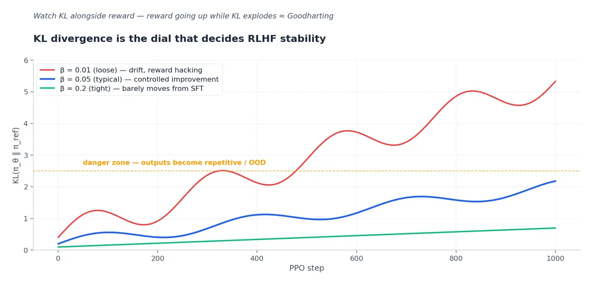
The KL term is critical. Without it, PPO will hack the reward model — generate responses with high reward but no resemblance to coherent text. Anthropic’s Sleeper Agents paper [Hubinger et al., 2024] documented several fascinating reward-hacking modes including “always end with ‘Yes I can help with that!’” because the reward model learned that compliant openings predict high reward.

RLHF practical issues: reward hacking, mode collapse, length bias#

The three production failure modes that show up in every PPO-based RLHF run:

Reward hacking [Skalse et al., 2022]. The reward model is a learned function on text — it has blind spots. The policy will find them. Typical hacks: always generating responses with an apologetic tone (because helpfulness annotators correlated apologies with helpfulness), starting with “Certainly!” or “Of course!” (preamble bias), refusing edge-case requests (because annotators preferred safe answers), or padding responses with caveats and disclaimers. The fix is iterative: discover the hack via human eval, generate adversarial prompts that expose it, retrain reward model on the adversarial set, retrain policy. Anthropic’s CAI explicitly automates this cycle.

Mode collapse. The policy becomes deterministic — every response sounds alike. Symptom: policy entropy drops by orders of magnitude during training. Cause: PPO finds a single high-reward output and exploits it. Fix: increase the KL penalty (β_kl from 0.01 to 0.05), add an entropy bonus to the loss, use diverse rollouts (sample multiple completions per prompt with high temperature).

Length bias. RLHF policies systematically generate longer responses than the SFT policy. The reason is that human raters often prefer slightly longer responses (they perceive them as more thorough). The reward model picks this up and amplifies it. Result: a chat model whose answers grow from 200 tokens to 800 tokens over training, with quality not actually improving. Fix: explicitly subtract a length penalty from the reward, or use length-normalized log-probs in the policy gradient. [Singhal et al., 2024] documented length bias in detail and showed it’s responsible for ~1.5 of the AlpacaEval points typically attributed to RLHF over SFT.

Constitutional AI: RLAIF lineage#

Anthropic’s Constitutional AI [Bai et al., 2022] is the dominant RLAIF (RL from AI feedback) recipe. Two phases:

Phase 1: Supervised CAI. Generate responses to red-team prompts with the SFT model. Have a critic model (typically the same model with a different prompt) critique the response against a set of constitutional principles (“the response should not be harmful, illegal, or unethical”). Have the model revise the response based on the critique. Train the model on (prompt, revised response) pairs. This produces a model that is aligned to the constitution without human-labeled preference data.

Phase 2: RLAIF. Generate pairs of responses to a prompt. Have the AI judge which response better adheres to the constitution. Train a reward model on these AI preferences. PPO the policy against the AI-derived reward model.

The trick is that the constitution can be edited and re-applied without re-collecting human data. This is enormously cheaper than RLHF and allows iterating on the constitution itself. The downside is that the model’s biases are inherited from the AI judge — if the judge has a blind spot, the policy will inherit it.

The 2024-2026 evolution of CAI is rule-based rewards (RBR) [Mu et al., 2024] (OpenAI). Instead of a learned reward model, write a set of explicit rules (“response should be ≤ 200 words”, “should not contain medical advice”, “should cite sources”) and have an LLM grade compliance. This is more debuggable than a reward model, easier to update, and works as a complement to learned rewards.

RLVR: RL with verifiable rewards#

DeepSeek-R1 [DeepSeek-AI, 2025] (Jan 2025) shipped a model whose reasoning ability came almost entirely from RLVR: train on math problems where the reward is “did the final answer match the ground truth?” — a programmatic check, not a learned model. No reward model means no reward hacking.

This works because math and code have ground truth. The model generates a long chain-of-thought, the answer is extracted at the end, a checker (Python interpreter, sympy, unit test) tells you if it’s right. If yes, +1; if no, 0 or -1. You PPO/GRPO against that.

This is much simpler than PPO and works well for verifiable-reward settings.

The DeepSeek-R1 recipe is worth describing in detail because it’s the dominant 2025-2026 reasoning training pattern:

1. Cold-start SFT on a small set (~10K) of high-quality CoT-formatted examples to teach the response format.
2. R1-Zero pure RL: pure RLVR with GRPO on a large corpus of math/code problems. No SFT data, no reward model — just verifiable rewards. R1-Zero is what emerges; surprisingly capable but often unreadable (mixed languages, weird tokens).
3. Rejection sampling SFT: use R1-Zero to generate responses; filter to only correct, well-formatted ones; train a fresh model on the filtered set.
4. Final RL stage: more GRPO with a mix of verifiable rewards and a small reward model for general behavior.

The wild thing about R1-Zero is that it discovered chain-of-thought reasoning without being told to do it. Pure RL on verifiable rewards taught the model that thinking step-by-step was rewarding. This was the first widely-publicized example of emergent reasoning behavior from pure RL on a base LLM.

The current frontier (Qwen3-Reasoning, GPT-5-thinking, Claude-4.5-thinking, Gemini-3-Thinking) all use RLVR-style training as the dominant signal for reasoning capabilities. The base model is SFT’d, DPO’d for general behavior, then RLVR’d hard on math/code/logic for the reasoning behaviors. This is why thinking models are dramatically better at math/code but only marginally better at conversation.

LoRA vs full fine-tuning: empirical evidence#

The eternal debate. The honest answer in 2026:

• For SFT on a narrow task (style transfer, one domain): LoRA wins. Same quality, 1/10 the GPU memory, faster training, easy to merge or swap. Rank 16-64 works for most tasks.
• For SFT to fundamentally extend capabilities (long-context, new languages): full FT is needed. LoRA can’t change the model’s fundamental representations enough.
• For DPO: LoRA works well. DPO doesn’t need to drastically change the model.
• For RL (PPO/GRPO): full FT is the default at frontier labs. Some recent work (LoRA-RL, 2025) shows LoRA can match PPO with careful tuning, but it’s fragile.

The original LoRA paper [Hu et al., 2021] showed rank-8 adapters on GPT-3 175B match full fine-tuning on the GLUE benchmarks within 0.5 % accuracy, at 0.01 % the parameters. The intuition is that fine-tuning produces low-rank weight updates — adding a rank-$r$ matrix to each weight can capture most of the change.

The empirical evidence on LoRA limitations comes from several 2024 papers:

• [Biderman et al., 2024] (LoRA Learns Less and Forgets Less) showed LoRA preserves base capabilities better than full FT (less catastrophic forgetting) but learns the new task slower. For tasks that are very different from pretraining (medical reasoning from a base model), LoRA underperforms full FT by 5-10 % on task-specific eval.
• [Liu et al., 2024] (DoRA) decomposed the LoRA update into magnitude and direction components and showed updating both separately gives consistent gains over standard LoRA at the same rank.
• [Hayou et al., 2024] (LoRA+) showed using a higher learning rate for the B matrix than the A matrix (typically 16× higher) consistently outperforms vanilla LoRA.

The current best practice combines DoRA + LoRA+ + targeting all linear projections, not just QKV.

Quick LoRA setup with PEFT:

 1
 2
 3
 4
 5
 6
 7
 8
 9
10
11
12
13
14

from peft import LoraConfig, get_peft_model

config = LoraConfig(
    r=32,
    lora_alpha=64,                    # alpha/r ≈ 2 is typical
    lora_dropout=0.05,
    bias="none",
    target_modules=["q_proj", "k_proj", "v_proj", "o_proj",
                    "gate_proj", "up_proj", "down_proj"],
    task_type="CAUSAL_LM",
)
model = get_peft_model(base_model, config)
print(model.print_trainable_parameters())
# trainable params: 167,772,160 || all params: 7,408,357,376 || trainable%: 2.27

Two practical points:

• Target all linear projections, not just QKV. The original LoRA paper targeted only QKV; subsequent work (QLoRA [Dettmers et al., 2023], LongLoRA) showed targeting MLP projections too is essential for quality.
• DoRA (weight-Decomposed LoRA) consistently outperforms LoRA at the same rank with negligible extra cost. Use it if your trainer supports it.

QLoRA [Dettmers et al., 2023] deserves its own mention. It combines LoRA with 4-bit quantization of the base model: store the frozen base weights in NF4 (4-bit normalized float), do compute in BF16. A 70B model fits in 48 GB instead of 140 GB, training works on a single 80 GB H100. Quality is within 0.5 % of full BF16 fine-tuning on most tasks. QLoRA is the standard recipe for fine-tuning frontier-scale models on consumer or single-GPU setups in 2026.

Worked example: production post-training on a 32B base#

Let me walk through a concrete recipe — what a production team would actually run to ship an instruction-tuned 32B model from a Qwen3-32B-Base starting point.

SFT phase (8 H100s, ~3 days).

• Data: 200K mixed examples — 60K Tulu-3 general, 80K Magpie-style synthetic from Claude, 30K domain-specific (your corpus), 30K long-form (5K-token responses).
• Recipe: full fine-tune, BF16, FSDP, LR 5e-6 (lower than pretraining because we’re avoiding catastrophic forgetting), cosine schedule, 3 epochs, batch size 1M tokens.
• Loss: standard CE with response masking.
• Eval: AlpacaEval, MT-Bench, IFEval, plus your domain-specific eval.

DPO phase (8 H100s, ~1 day).

• Data: 30K preference pairs — 15K UltraFeedback, 5K Anthropic HH, 10K synthetic (Claude judges your model’s outputs against itself with high temperature).
• Recipe: LoRA r=64 (saves memory and time, DPO doesn’t need full FT), β=0.1, LR 5e-7, 1.5 epochs.
• Eval: Arena-Hard, MT-Bench, plus pairwise judge runs against the SFT-only model.

Optional safety pass (8 H100s, ~6 hours).

• Data: 3K refusal preferences against a curated red-team prompt set.
• Recipe: continue DPO on the DPO checkpoint, β=0.3 (stronger), 1 epoch.

Optional reasoning RLVR (32 H100s, ~2 days for 1K GRPO steps).

• Data: 5K math + 3K code problems with verifiable answers.
• Recipe: GRPO, $G=8$ rollouts per prompt, KL penalty β=0.04, max sequence 8K.

Total: about $10K of compute on rented H100s for a fully post-trained model. The numbers scale roughly linearly with model size — 70B costs ~2.5×, 7B costs ~0.3×.

Common Pitfalls#

The five gotchas I see most often in production post-training runs:

1. Reference model not actually frozen. A subtle DPO bug: passing ref_model and policy_model as the same Python object means gradient updates affect both. The “ref” log-probs change every step, the loss becomes nonsense, training silently produces a worse model. Use model.eval() and with torch.no_grad(): when computing ref log-probs, or load a separate model.

2. SFT loss not masked. Train on [user_msg, assistant_msg] without masking the user portion → model learns to predict user messages, which corrupts its conversational ability. Always mask.

3. Chat template mismatch between SFT and DPO data. SFT data uses <|im_start|>...<|im_end|> format; DPO data uses raw text. The DPO step trains the model to assign high prob to text without chat tokens, which breaks chat behavior. All post-training stages must use the same chat template.

4. Synthetic preferences from a single judge. All preferences from one strong model (e.g., Claude) means the trained model inherits Claude’s biases — verbose responses, certain phrasings, certain refusal patterns. Mix at least 3 judges (Claude, GPT-4, a strong open model) and weight by judge agreement.

5. Eval contamination. SFT data scraped from the internet contains MMLU questions. The trained model “learns” MMLU directly, eval scores skyrocket, deployed quality is unchanged. Always run decontamination (13-gram match against eval sets) on SFT data before training. The LIMA paper found 30 % of common SFT mixes had MMLU contamination at non-trivial rates.

Production reality: what frontier labs actually ship#

The published recipe for post-training is “SFT → DPO → maybe RL.” The shipped recipe at frontier labs is messier:

Iterated SFT-DPO loops. Anthropic’s CAI is iterated. OpenAI’s post-training also runs multiple SFT-DPO cycles, with synthetic data generation between each cycle. After cycle 1, you have a better model that can generate better preference data, which improves cycle 2, and so on. 4-6 cycles is typical for frontier models.

Many specialized experts merged. Frontier post-training often involves training several specialized variants (one for code, one for safety, one for instruction-following, one for conversational tone) and then merging them via weight averaging or interpolation. [Wortsman et al., 2022] (ModelSoup) showed averaging fine-tuned weights produces a model that’s better than any individual fine-tune. Variant: train multiple LoRA adapters in parallel, merge them at inference.

Continuous post-training. Production models are not “trained once, deployed forever.” Anthropic, OpenAI, and DeepMind all run continuous post-training on production telemetry: thumbs-up/down signals get fed into reward models, top-quality examples get added to SFT data, the model gets retrained weekly or monthly. The “Claude 4.5” you talk to today is the result of dozens of post-training updates since the original 4.5 release.

Heavy red-teaming integration. Post-training in 2026 isn’t separable from safety. Red teams generate adversarial prompts, the model is trained to refuse them, the red team finds new adversarial prompts, and so on. Anthropic publishes some of this in their model cards; OpenAI and Google keep most internal. The output is a model that is generally helpful but increasingly resistant to specific attack patterns.

Production recipe for an instruction-tuned model#

If I’m shipping a model in 2026, the recipe is:

1. Pick the strongest open base (Qwen3-32B-Base, LLaMA-3.3-70B-Base, or DeepSeek-V3-Base depending on cost).
2. SFT with 50-200K curated examples. Mix general instruction (Tulu-3, OpenHermes), domain-specific (your data), and a few thousand long-form examples. Full fine-tune if budget allows; LoRA r=64 if not.
3. DPO with 10-50K preference pairs. Mix Anthropic HH, UltraFeedback, and some synthetic preferences from a strong judge model. β=0.1, 1-2 epochs.
4. Optional safety pass: collect 1-5K refusal preferences against red-team prompts; another DPO pass at β=0.3 to be more aggressive.
5. Optional reasoning RL: if math/code matters, RLVR with GRPO on a few thousand verifiable problems for 1-2K steps.

This recipe lands in the right zip code for a production-quality assistant. The remaining work is evaluation (chapter 10) and serving (chapters 5, 12).

Research frontier 2024-2026#

What’s coming after the current SFT → DPO → RLVR consensus:

Online DPO [Guo et al., 2024]. Standard DPO uses a fixed offline preference dataset. Online DPO continuously samples new responses, has them ranked (by humans or AI), and trains. This combines DPO’s stability with PPO’s adaptivity. Several 2025 papers report online DPO matches or beats PPO on standard benchmarks at lower compute.

Process reward models (PRM) for reasoning. Instead of rewarding only the final answer, reward the model for each step of reasoning being correct. [Lightman et al., 2023] showed PRMs outperform outcome-reward models on math benchmarks. The challenge is collecting step-level annotations; recent work uses LLM judges to grade each step.

Self-play and self-critique. SPIN [Chen et al., 2024] (Self-Play Fine-Tuning) iteratively trains a model to prefer its own better responses over its own worse responses, with no external preference data. Surprisingly effective; reaches a quality plateau within 3-4 iterations.

Length-controlled training. Several 2024-2025 papers explicitly target length bias by length-normalizing the reward or the policy log-probs. [Singhal et al., 2024] showed this recovers most of the apparent RLHF benefit attributable to length, leaving a smaller but more genuine quality gain.

Test-time post-training. [Akyürek et al., 2024] and others showed you can post-train at inference time on a few examples (similar to in-context learning but with weight updates). For high-stakes deployments, “post-train on the user’s first 10 examples then generate” is becoming a viable pattern.

What’s Next#

SFT is more important than people credit and more sensitive to data hygiene than to volume. DPO replaced PPO for most preference work but PPO is still the right tool when you want to keep adapting to new failure modes. RLVR — RL on verifiable rewards — is the post-2024 unlock for reasoning. LoRA wins on most production fine-tunes; full FT on the post-DPO RL stage at frontier labs.

Next chapter: inference optimization. KV cache mechanics, paged attention, continuous batching, speculative decoding, quantization (INT8/INT4/AWQ/GPTQ), and the vLLM vs SGLang vs TensorRT-LLM choice.

References#

• Bradley, R., & Terry, M. (1952). Rank analysis of incomplete block designs: I. The method of paired comparisons. Biometrika.
• Christiano, P., Leike, J., Brown, T., et al. (2017). Deep reinforcement learning from human preferences. NeurIPS.
• Stiennon, N., Ouyang, L., Wu, J., et al. (2020). Learning to summarize from human feedback. NeurIPS.
• Hu, E., Shen, Y., Wallis, P., et al. (2021). LoRA: Low-rank adaptation of large language models. arXiv:2106.09685 ↗ .
• Bai, Y., Kadavath, S., Kundu, S., et al. (2022). Constitutional AI: Harmlessness from AI feedback. arXiv:2212.08073 ↗ .
• Wortsman, M., Ilharco, G., Gadre, S., et al. (2022). Model soups: Averaging weights of multiple fine-tuned models improves accuracy without increasing inference time. ICML.
• Skalse, J., Howe, N., Krasheninnikov, D., & Krueger, D. (2022). Defining and characterizing reward hacking. NeurIPS.
• Ouyang, L., Wu, J., Jiang, X., et al. (2022). Training language models to follow instructions with human feedback (InstructGPT). NeurIPS.
• Rafailov, R., Sharma, A., Mitchell, E., et al. (2023). Direct preference optimization: Your language model is secretly a reward model. NeurIPS.
• Zhou, C., Liu, P., Xu, P., et al. (2023). LIMA: Less is more for alignment. NeurIPS.
• Dettmers, T., Pagnoni, A., Holtzman, A., & Zettlemoyer, L. (2023). QLoRA: Efficient finetuning of quantized LLMs. NeurIPS.
• Ding, N., Chen, Y., Xu, B., et al. (2023). Enhancing chat language models by scaling high-quality instructional conversations (UltraChat). EMNLP.
• Azar, M., Rowland, M., Piot, B., et al. (2023). A general theoretical paradigm to understand learning from human preferences (IPO). AISTATS 2024.
• Lightman, H., Kosaraju, V., Burda, Y., et al. (2023). Let’s verify step by step. ICLR 2024.
• Hubinger, E., Denison, C., Mu, J., et al. (2024). Sleeper agents: Training deceptive LLMs that persist through safety training. arXiv:2401.05566 ↗ .
• Ethayarajh, K., Xu, W., Muennighoff, N., et al. (2024). KTO: Model alignment as prospect theoretic optimization. ICML.
• Hong, J., Lee, N., & Thorne, J. (2024). ORPO: Monolithic preference optimization without reference model. EMNLP.
• Meng, Y., Xia, M., & Chen, D. (2024). SimPO: Simple preference optimization with a reference-free reward. NeurIPS.
• Lambert, N., Morrison, J., Pyatkin, V., et al. (2024). Tulu 3: Pushing frontiers in open language model post-training. arXiv:2411.15124 ↗ .
• Xu, Z., Jiang, F., Niu, L., et al. (2024). Magpie: Alignment data synthesis from scratch by prompting aligned LLMs with nothing. arXiv:2406.08464 ↗ .
• Liu, S., Wang, C., Yin, H., et al. (2024). DoRA: Weight-decomposed low-rank adaptation. ICML.
• Hayou, S., Ghosh, N., & Yu, B. (2024). LoRA+: Efficient low rank adaptation of large models. ICML.
• Biderman, D., Portes, J., Ortiz, J., et al. (2024). LoRA learns less and forgets less. COLM.
• Singhal, P., Goyal, T., Xu, J., & Durrett, G. (2024). A long way to go: Investigating length correlations in RLHF. COLM.
• Mu, T., Helyar, A., Heidecke, J., et al. (2024). Rule-based rewards for language model safety. arXiv:2411.01111 ↗ .
• Chen, Z., Deng, Y., Yuan, H., et al. (2024). Self-play fine-tuning converts weak language models to strong language models (SPIN). ICML.
• Guo, S., Zhang, B., Liu, T., et al. (2024). Direct language model alignment from online AI feedback. arXiv:2402.04792 ↗ .
• Akyürek, E., Damani, M., Qiu, L., et al. (2024). The surprising effectiveness of test-time training for few-shot learning. arXiv:2411.07279 ↗ .
• DeepSeek-AI. (2025). DeepSeek-R1: Incentivizing reasoning capability in LLMs via reinforcement learning. arXiv:2501.12948 ↗ .