NLP Part 3: RNN and Sequence Modeling

Open Google Translate, swipe-type a message, dictate a memo to your phone — every one of these systems must consume an ordered stream of tokens and produce another. A feed-forward network treats each input independently, but language is fundamentally sequential: the meaning of “mat” in the cat sat on the mat depends on every word that came before. Recurrent Neural Networks (RNNs) handle this by maintaining a hidden state that evolves as they consume each token. The hidden state is the network’s running summary of the past — its memory.

This article builds up the family of recurrent architectures from scratch. We start with the vanilla RNN, derive why it cannot remember more than a dozen tokens, watch the LSTM and GRU rescue it with gating, and finish with a working English-to-French translator in PyTorch. By the end, you will understand the architectural shift that ultimately motivated attention and Transformers.

What you will learn

How RNNs maintain memory through recurrent connections and parameter sharing
A first-principles derivation of vanishing and exploding gradients
How LSTM gates (forget, input, output) and the cell-state highway fix long-range dependencies
GRU as a leaner alternative to LSTM, and when to pick each
Bidirectional and stacked RNNs for richer per-token representations
The Seq2Seq encoder-decoder, its bottleneck, and why attention was inevitable
Working PyTorch implementations of text generation and translation

Prerequisites: Parts 1-2 of this series (tokenization and embeddings), plus basic PyTorch (tensors, nn.Module, training loops).

Vanilla RNN unrolled across five time steps, showing recurrent weight sharing

At every time step $t$, an RNN consumes input $x_t$ and the previous hidden state $h_{t-1}$, then produces a new hidden state and an output:

$$ h_t = \tanh(W_h h_{t-1} + W_x x_t + b), \qquad y_t = W_y h_t + b_y. $$

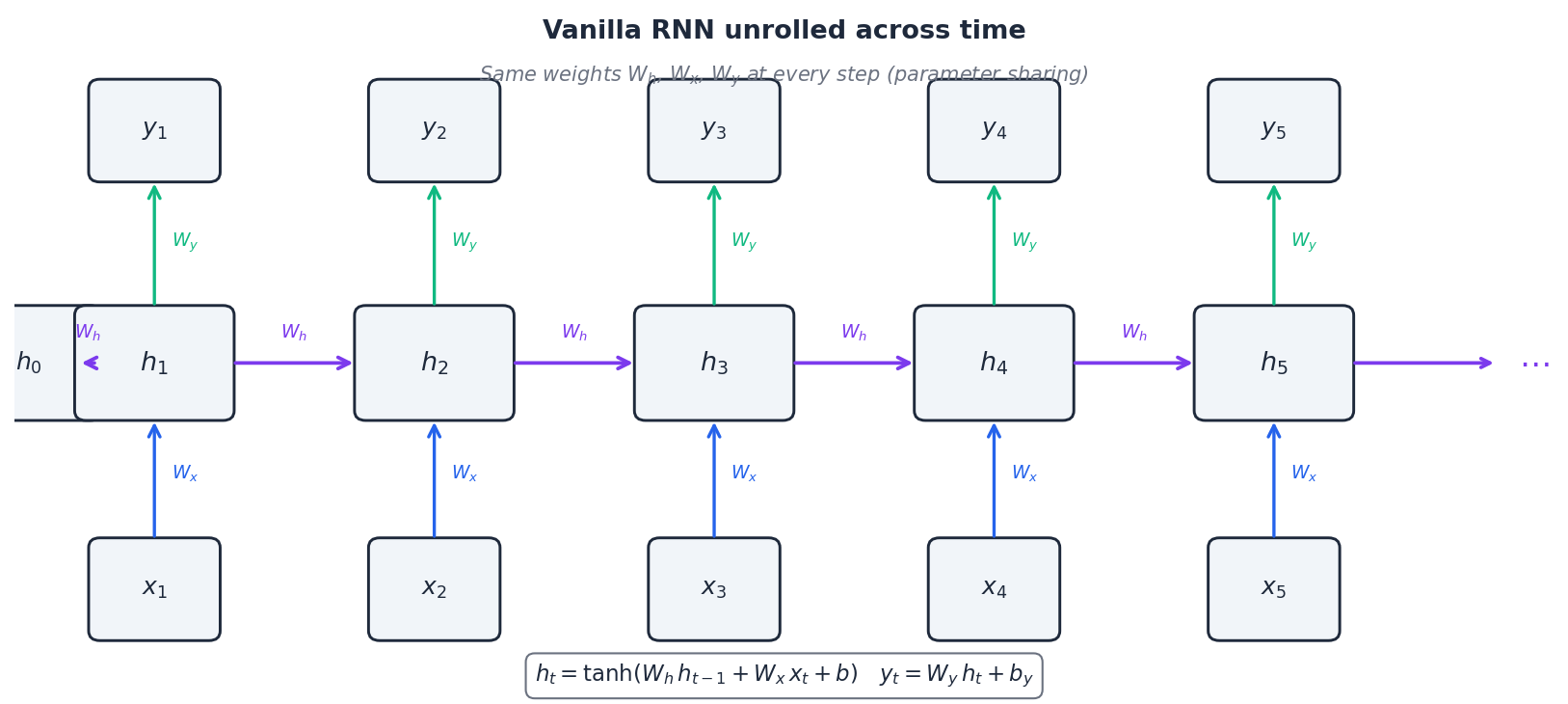
The crucial property — visible in the figure as the same arrows repeating at each step — is that the matrices $W_h$, $W_x$, $W_y$ are reused at every position. This single design choice gives RNNs three nice features at once:

Generalisation across positions: a pattern learned at position 3 transfers to position 30, because the same weights see both.
Constant parameter count: the model size is independent of sequence length, so a 10-token and a 10 000-token sentence cost the same to store.
Variable-length input and output: nothing in the equations cares whether $T$ is 5 or 500.

Mentally, picture the network reading one token at a time, updating its “running understanding” of the sentence after each word. The hidden state at step $t$ is a learned, fixed-size summary of $x_1, \dots, x_t$.

2. The vanishing gradient problem

Gradient norm decay vs. distance, with a long-range dependency illustrated on a sample sentence

The trouble starts when we train. To compute gradients we unroll the network through time and run backpropagation — a procedure called Backpropagation Through Time (BPTT). The gradient of the loss at step $T$ with respect to the hidden state at step $t$ is a chain product:

$$ \frac{\partial h_T}{\partial h_t} \;=\; \prod_{k=t}^{T-1} \frac{\partial h_{k+1}}{\partial h_k}. $$

Each Jacobian factor in that product is roughly $W_h^{\top}\,\mathrm{diag}(\tanh'(\cdot))$. Because $\tanh' \le 1$, the factor’s spectral norm is bounded above by the largest singular value of $W_h$, call it $\lambda$. Multiplying $T-t$ such factors gives

$$ \left\| \frac{\partial h_T}{\partial h_t} \right\| \;\lesssim\; \lambda^{\,T-t}. $$

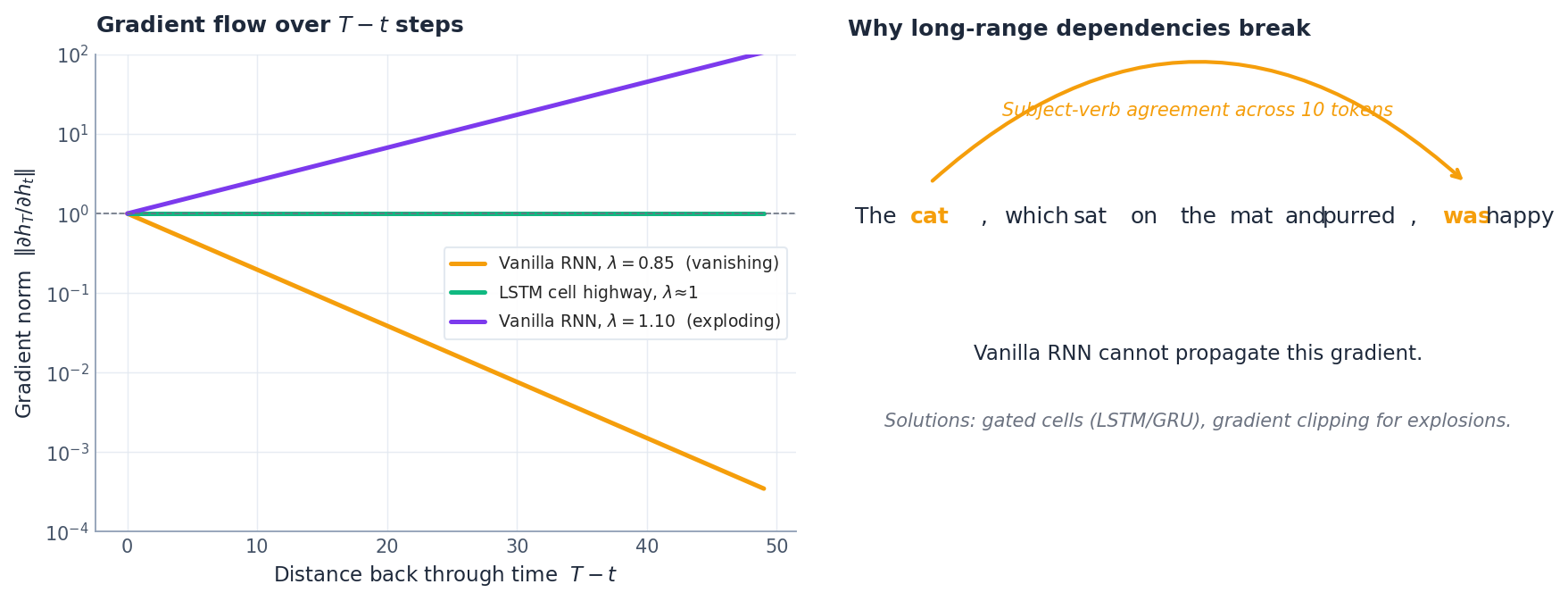
Two regimes follow immediately, and you can see both in the left panel of the figure:

If $\lambda < 1$, the gradient norm decays exponentially. Beyond roughly 10–20 steps the signal is numerically zero, so the optimiser cannot tell that token $t$ matters for the loss at $T$. The model literally cannot learn the dependency.
If $\lambda > 1$, the gradient explodes — finite weight updates become wild, and training diverges in a single step.

The right panel makes this concrete. In “The cat, which sat on the mat and purred, was happy”, subject (“cat”) and verb (“was”) are separated by ten tokens. A vanilla RNN cannot route the gradient that far, so it never learns the agreement.

What helps in practice. Gradient clipping — capping the global norm at some threshold like 5.0 — solves explosion but does nothing for vanishing. The real fix requires re-architecting the recurrence so that gradients have a path that does not shrink. That path is exactly what LSTMs and GRUs introduce.

3. Long Short-Term Memory (LSTM)

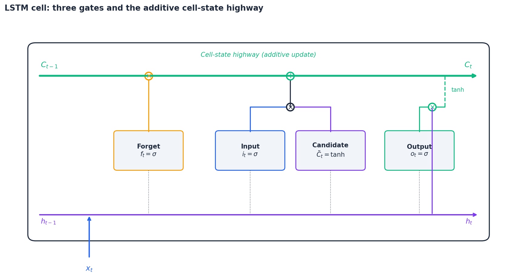
LSTM cell architecture: forget, input, output gates and the additive cell-state highway

The LSTM (Hochreiter & Schmidhuber, 1997) replaces the simple recurrent unit with a gated cell that carries an explicit long-term memory $C_t$ alongside the hidden state $h_t$.

The three gates

Let $[h_{t-1}, x_t]$ denote the concatenation of the previous hidden state and current input. All gates share this same input.

Forget gate — what to discard from the long-term memory:

$$f_t = \sigma(W_f [h_{t-1}, x_t] + b_f).$$

Input gate + candidate — what new information to write:

$$ i_t = \sigma(W_i [h_{t-1}, x_t] + b_i), \qquad \tilde{C}_t = \tanh(W_C [h_{t-1}, x_t] + b_C). $$

Cell-state update — combine old memory with new content:

$$C_t = f_t \odot C_{t-1} + i_t \odot \tilde{C}_t.$$

Output gate — what slice of the cell to expose as the new hidden state:

$$ o_t = \sigma(W_o [h_{t-1}, x_t] + b_o), \qquad h_t = o_t \odot \tanh(C_t). $$

Here $\sigma$ is the sigmoid (a soft 0–1 switch) and $\odot$ is element-wise multiplication. Each gate is a learned, position-dependent decision: forget this, write that, expose the rest.

Why this fixes vanishing gradients

The cell-state line in the diagram is the key. Its update is additive:

$$C_t = f_t \odot C_{t-1} + i_t \odot \tilde{C}_t.$$

Differentiating gives $\partial C_t / \partial C_{t-1} = f_t$, an element-wise scalar in $[0,1]$. When the forget gate stays near 1, the chain product $\prod f_k$ stays near 1 too — gradients flow through the cell-state highway essentially unchanged, even over hundreds of steps. Compare this with the vanilla RNN’s multiplicative update through $W_h$, which compounds toward zero. The LSTM trades one shared $W_h$ for a learnable, time-varying $f_t$, and that single change is what lets it model long contexts.

The conveyor-belt analogy

Picture the cell state as a conveyor belt running the length of the sequence. The forget gate is a worker who removes items the belt no longer needs, the input gate is a worker who places new items on, and the output gate is a window that decides which items the outside world (the rest of the network) sees right now. An item placed at step 3 can ride the belt undisturbed all the way to step 300.

4. Gated Recurrent Unit (GRU)

GRU cell with reset and update gates — simpler than LSTM

The GRU (Cho et al., 2014) keeps the gating idea but trims the design. It merges forget and input into a single update gate, drops the separate cell state, and works directly on $h_t$:

$$ z_t = \sigma(W_z [h_{t-1}, x_t]), \qquad r_t = \sigma(W_r [h_{t-1}, x_t]), $$$$ \tilde{h}_t = \tanh(W [r_t \odot h_{t-1}, x_t]), \qquad h_t = (1 - z_t) \odot h_{t-1} + z_t \odot \tilde{h}_t. $$

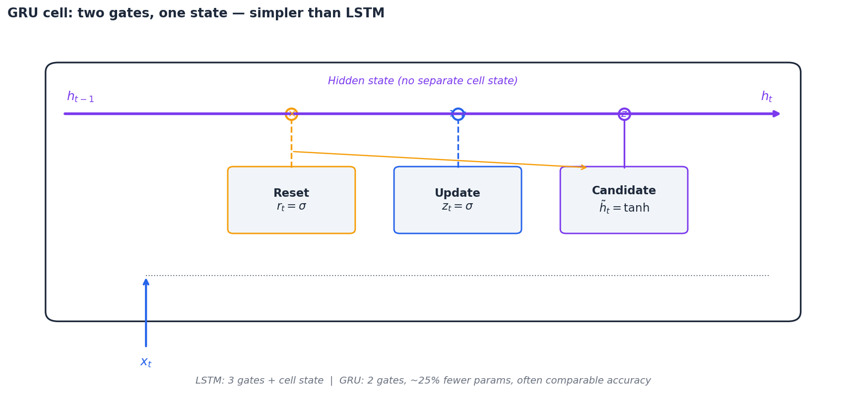
The reset gate $r_t$ controls how much of the past leaks into the candidate. The update gate $z_t$ does linear interpolation between the old state and the new candidate — when $z_t \approx 0$, the GRU just copies $h_{t-1}$ forward, which is exactly the same gradient-preserving trick as the LSTM’s cell highway.

LSTM vs. GRU

Aspect	LSTM	GRU
Gates	3 (forget, input, output)	2 (reset, update)
Separate cell state	Yes ($C_t$)	No (just $h_t$)
Parameters	$\sim\!4\times$ vanilla RNN	$\sim\!3\times$ vanilla RNN ($\approx 25\%$ fewer than LSTM)
Long sequences	Slight edge in many benchmarks	Comparable
Training speed	Slower	Faster

Rule of thumb: start with a GRU. It trains faster, has fewer hyperparameters, and on most tasks the accuracy gap is within noise. Switch to LSTM if your sequences are very long or if your task is known to benefit from the extra capacity (some speech tasks do).

5. Bidirectional RNNs

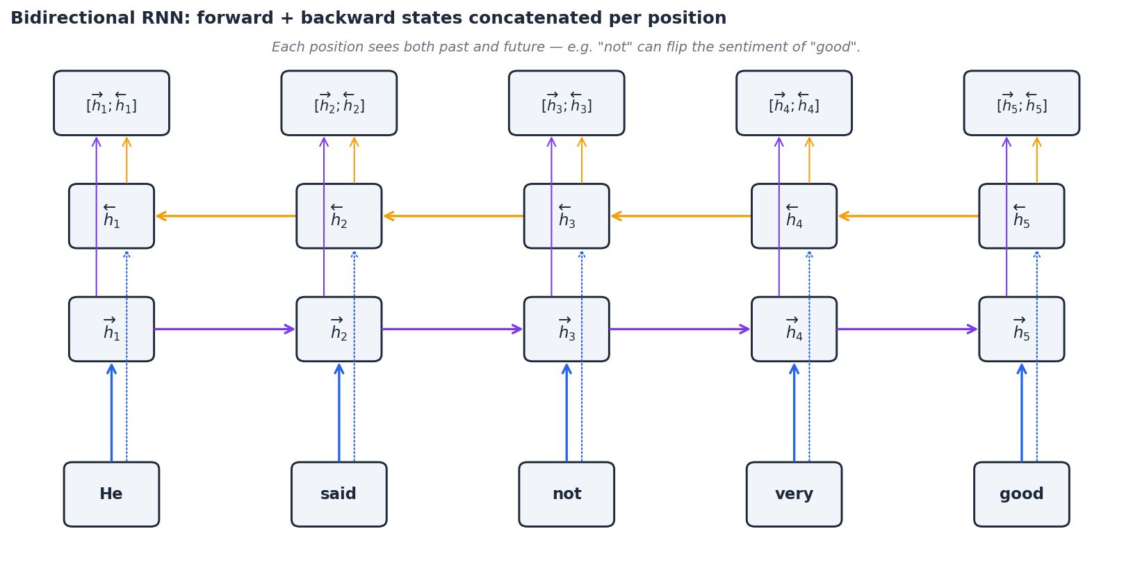
Bidirectional RNN: forward and backward states concatenated per position

In many tasks, the future is just as informative as the past. “He said the food was not good” — without seeing “not”, a left-to-right reader would label “good” as positive sentiment.

A Bidirectional RNN (Schuster & Paliwal, 1997) runs two independent recurrences and concatenates their states:

$$ \overrightarrow{h}_t = \mathrm{RNN}_\text{fwd}(x_t, \overrightarrow{h}_{t-1}), \qquad \overleftarrow{h}_t = \mathrm{RNN}_\text{bwd}(x_t, \overleftarrow{h}_{t+1}), $$$$ h_t = \big[\overrightarrow{h}_t \,;\, \overleftarrow{h}_t\big]. $$

Each per-position representation now sees both directions of context.

Use it for: named entity recognition, part-of-speech tagging, machine-translation encoders, anything where you have the whole input up front.

Do not use it for: streaming or autoregressive generation. The backward pass requires future tokens, which by definition do not exist when you are emitting one token at a time.

6. Stacked RNNs

Depth helps: stacking RNN layers lets each layer build on the previous layer’s per-step output:

$$ h_t^{(1)} = \mathrm{RNN}^{(1)}(x_t,\, h_{t-1}^{(1)}), \qquad h_t^{(2)} = \mathrm{RNN}^{(2)}(h_t^{(1)},\, h_{t-1}^{(2)}). $$

Empirically the lower layers learn local patterns (character n-grams, word boundaries, morphology), while the higher layers capture syntax and longer-range semantics. Two to four layers is the sweet spot for most NLP tasks; beyond that, residual connections become essential to keep optimisation stable.

7. Sequence-to-sequence models

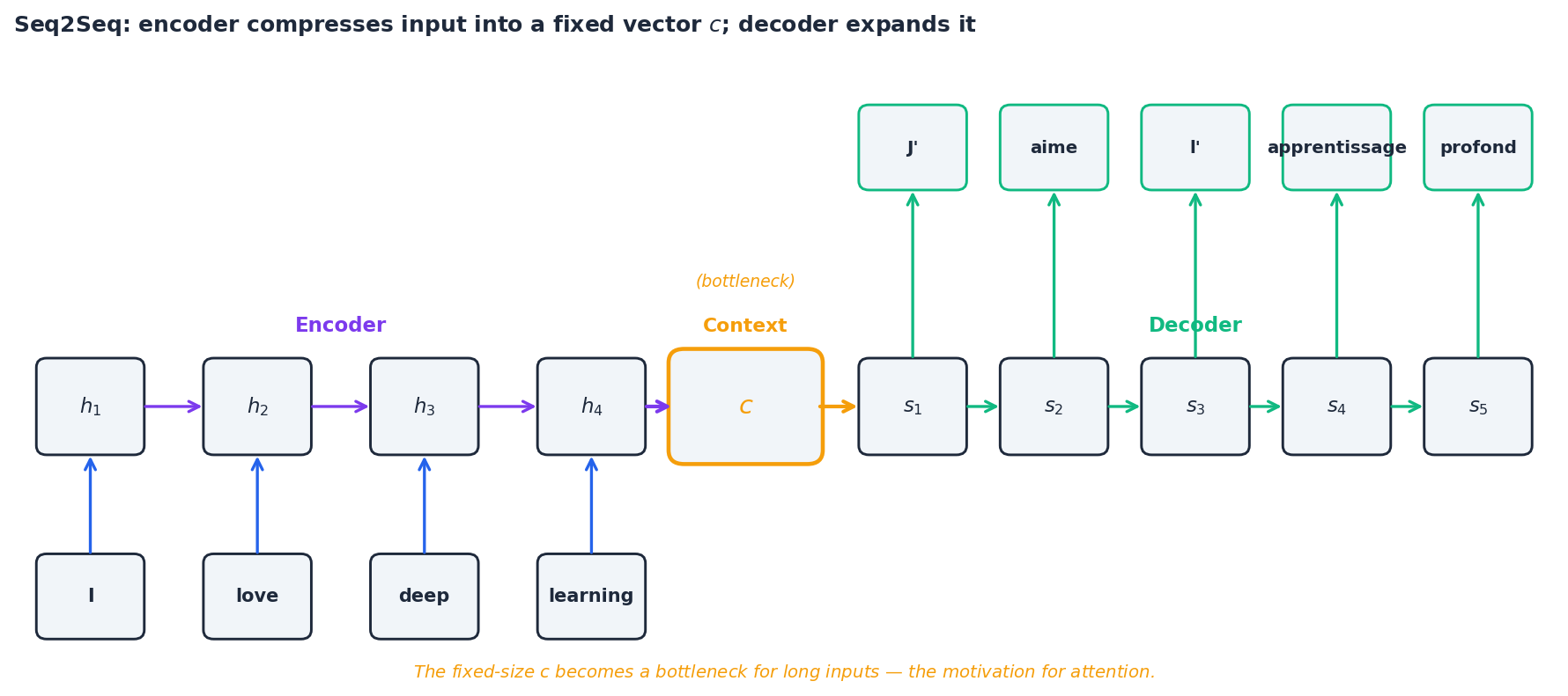
Seq2Seq encoder-decoder with the fixed-size context-vector bottleneck

The Seq2Seq architecture (Sutskever et al., 2014) maps an input sequence to an output sequence of different length — the canonical example being machine translation. It uses two RNNs:

An encoder reads the entire input and compresses it into a single context vector $c = h_T^{\text{enc}}$.
A decoder generates the output one token at a time, conditioned on $c$ and on the tokens it has already emitted:

$$ s_t = \mathrm{RNN}_\text{dec}(y_{t-1}, s_{t-1}), \qquad P(y_t \mid y_{The bottleneck. The whole input — possibly 50 words of context — must squeeze through the single fixed-size vector $c$. For short sentences this is fine; for long ones, the encoder simply runs out of room. Sutskever’s original paper found that BLEU scores fell sharply once the input exceeded about 30 tokens, and that reversing the source sentence helped (which is itself a hint that the bottleneck was the problem).

This bottleneck is the direct motivation for attention, the topic of Part 4: instead of forcing the decoder to live on a single $c$, attention lets it look back at every encoder hidden state at each decoding step.

8. PyTorch implementation: character-level text generator

Let us train a tiny LSTM that learns to generate text one character at a time.

Dataset preparation

 1
 2
 3
 4
 5
 6
 7
 8
 9
10
11
12
13
14
import torch
import torch.nn as nn
import numpy as np

text = """Deep learning is a subset of machine learning that uses neural
networks with many layers. These networks can learn hierarchical
representations of data, making them powerful for tasks like image
recognition, natural language processing, and speech recognition."""

chars = sorted(set(text))
char_to_idx = {ch: i for i, ch in enumerate(chars)}
idx_to_char = {i: ch for i, ch in enumerate(chars)}
vocab_size = len(chars)
print(f"Vocabulary size: {vocab_size} characters")

Model

 1
 2
 3
 4
 5
 6
 7
 8
 9
10
11
12
13
14
15
16
17
18
19
class CharRNN(nn.Module):
    def __init__(self, vocab_size, hidden_size, num_layers):
        super().__init__()
        self.hidden_size = hidden_size
        self.num_layers = num_layers
        self.embedding = nn.Embedding(vocab_size, hidden_size)
        self.lstm = nn.LSTM(hidden_size, hidden_size, num_layers, batch_first=True)
        self.fc = nn.Linear(hidden_size, vocab_size)

    def forward(self, x, hidden):
        embedded = self.embedding(x)
        out, hidden = self.lstm(embedded, hidden)
        out = self.fc(out.reshape(-1, self.hidden_size))
        return out, hidden

    def init_hidden(self, batch_size, device):
        h0 = torch.zeros(self.num_layers, batch_size, self.hidden_size).to(device)
        c0 = torch.zeros(self.num_layers, batch_size, self.hidden_size).to(device)
        return (h0, c0)

Training loop

 1
 2
 3
 4
 5
 6
 7
 8
 9
10
11
12
13
14
15
16
17
18
19
20
21
22
23
24
25
26
27
28
29
30
def train(model, text_data, epochs=100, seq_length=50, batch_size=16, lr=0.002):
    device = torch.device('cuda' if torch.cuda.is_available() else 'cpu')
    model = model.to(device)
    criterion = nn.CrossEntropyLoss()
    optimizer = torch.optim.Adam(model.parameters(), lr=lr)
    data = [char_to_idx[ch] for ch in text_data]

    for epoch in range(epochs):
        model.train()
        hidden = model.init_hidden(batch_size, device)
        total_loss = 0
        n_batches = len(data) // (seq_length * batch_size)

        for _ in range(n_batches):
            starts = np.random.randint(0, len(data) - seq_length - 1, batch_size)
            inputs = torch.LongTensor([data[s:s+seq_length] for s in starts]).to(device)
            targets = torch.LongTensor([data[s+1:s+seq_length+1] for s in starts]).to(device)

            hidden = tuple(h.detach() for h in hidden)        # truncated BPTT
            outputs, hidden = model(inputs, hidden)
            loss = criterion(outputs, targets.reshape(-1))

            optimizer.zero_grad()
            loss.backward()
            torch.nn.utils.clip_grad_norm_(model.parameters(), 5.0)   # explosion guard
            optimizer.step()
            total_loss += loss.item()

        if (epoch + 1) % 20 == 0:
            print(f"Epoch {epoch+1}/{epochs}, Loss: {total_loss/n_batches:.4f}")

Note the two RNN-specific tricks: detaching hidden state between batches to truncate BPTT (otherwise gradients try to flow back through the entire training corpus), and gradient clipping to defuse the exploding-gradient regime.

Sampling — temperature controls creativity

 1
 2
 3
 4
 5
 6
 7
 8
 9
10
11
12
13
14
15
16
17
18
19
20
21
22
23
24
25
def generate(model, start_str, length=200, temperature=0.8):
    device = next(model.parameters()).device
    model.eval()
    hidden = model.init_hidden(1, device)
    input_seq = [char_to_idx[ch] for ch in start_str]
    generated = start_str

    with torch.no_grad():
        for idx in input_seq[:-1]:                     # warm up the hidden state
            x = torch.LongTensor([[idx]]).to(device)
            _, hidden = model(x, hidden)

        x = torch.LongTensor([[input_seq[-1]]]).to(device)
        for _ in range(length):
            output, hidden = model(x, hidden)
            probs = torch.softmax(output.squeeze() / temperature, dim=0).cpu().numpy()
            char_idx = np.random.choice(len(probs), p=probs)
            generated += idx_to_char[char_idx]
            x = torch.LongTensor([[char_idx]]).to(device)

    return generated

model = CharRNN(vocab_size, hidden_size=128, num_layers=2)
train(model, text, epochs=100)
print(generate(model, "Deep learning", length=200))

Temperature rescales logits before softmax: $P(w) = \mathrm{softmax}(\text{logits}/T)$. Low $T$ (around 0.5) sharpens the distribution toward the mode and yields conservative, repetitive output. High $T$ (1.5+) flattens it and produces creative but often nonsensical text. $T=0.8$ is a common compromise.

9. PyTorch implementation: a minimal Seq2Seq translator

A bare-bones English-to-French translator, useful for understanding the encoder-decoder pipeline before we add attention in Part 4.

Data and vocabulary

 1
 2
 3
 4
 5
 6
 7
 8
 9
10
11
12
13
14
15
16
17
18
19
20
21
22
23
24
25
26
27
28
29
30
import torch
import torch.nn as nn
import random

pairs = [
    ("hello", "bonjour"), ("good morning", "bon matin"),
    ("thank you", "merci"), ("goodbye", "au revoir"),
    ("how are you", "comment allez vous"),
    ("i love you", "je t aime"), ("welcome", "bienvenue"),
]

SOS, EOS = 0, 1

class Vocab:
    def __init__(self):
        self.word2idx = {"<SOS>": SOS, "<EOS>": EOS}
        self.idx2word = {SOS: "<SOS>", EOS: "<EOS>"}
        self.n_words = 2

    def add_sentence(self, sentence):
        for word in sentence.split():
            if word not in self.word2idx:
                self.word2idx[word] = self.n_words
                self.idx2word[self.n_words] = word
                self.n_words += 1

src_vocab, tgt_vocab = Vocab(), Vocab()
for en, fr in pairs:
    src_vocab.add_sentence(en)
    tgt_vocab.add_sentence(fr)

Encoder and decoder

 1
 2
 3
 4
 5
 6
 7
 8
 9
10
11
12
13
14
15
16
17
18
19
class Encoder(nn.Module):
    def __init__(self, vocab_size, hidden_size):
        super().__init__()
        self.embedding = nn.Embedding(vocab_size, hidden_size)
        self.lstm = nn.LSTM(hidden_size, hidden_size, batch_first=True)

    def forward(self, x):
        return self.lstm(self.embedding(x))

class Decoder(nn.Module):
    def __init__(self, hidden_size, vocab_size):
        super().__init__()
        self.embedding = nn.Embedding(vocab_size, hidden_size)
        self.lstm = nn.LSTM(hidden_size, hidden_size, batch_first=True)
        self.fc = nn.Linear(hidden_size, vocab_size)

    def forward(self, x, hidden):
        out, hidden = self.lstm(self.embedding(x), hidden)
        return self.fc(out.squeeze(1)), hidden

Training (with teacher forcing)

 1
 2
 3
 4
 5
 6
 7
 8
 9
10
11
12
13
14
15
16
17
18
19
20
21
22
23
24
25
26
27
28
29
30
31
32
33
34
def train_seq2seq(encoder, decoder, pairs, epochs=500, lr=0.01):
    device = torch.device('cuda' if torch.cuda.is_available() else 'cpu')
    encoder, decoder = encoder.to(device), decoder.to(device)
    enc_opt = torch.optim.Adam(encoder.parameters(), lr=lr)
    dec_opt = torch.optim.Adam(decoder.parameters(), lr=lr)
    criterion = nn.CrossEntropyLoss()

    for epoch in range(epochs):
        total_loss = 0
        random.shuffle(pairs)
        for src_sent, tgt_sent in pairs:
            src_ids = [src_vocab.word2idx[w] for w in src_sent.split()] + [EOS]
            tgt_ids = [tgt_vocab.word2idx[w] for w in tgt_sent.split()] + [EOS]

            src_t = torch.LongTensor([src_ids]).to(device)
            tgt_t = torch.LongTensor(tgt_ids).to(device)

            enc_opt.zero_grad(); dec_opt.zero_grad()

            _, hidden = encoder(src_t)                     # context vector
            dec_input = torch.LongTensor([[SOS]]).to(device)
            loss = 0

            for i in range(len(tgt_ids)):
                output, hidden = decoder(dec_input, hidden)
                loss += criterion(output, tgt_t[i:i+1])
                dec_input = tgt_t[i:i+1].unsqueeze(0)      # teacher forcing

            loss.backward()
            enc_opt.step(); dec_opt.step()
            total_loss += loss.item() / len(tgt_ids)

        if (epoch + 1) % 100 == 0:
            print(f"Epoch {epoch+1}/{epochs}, Loss: {total_loss/len(pairs):.4f}")

Inference

 1
 2
 3
 4
 5
 6
 7
 8
 9
10
11
12
13
14
15
16
17
18
19
20
21
22
23
def translate(encoder, decoder, sentence):
    device = next(encoder.parameters()).device
    encoder.eval(); decoder.eval()
    with torch.no_grad():
        src_ids = [src_vocab.word2idx.get(w, 0) for w in sentence.split()] + [EOS]
        _, hidden = encoder(torch.LongTensor([src_ids]).to(device))
        dec_input = torch.LongTensor([[SOS]]).to(device)
        words = []
        for _ in range(20):
            output, hidden = decoder(dec_input, hidden)
            token = output.argmax(dim=-1).item()
            if token == EOS:
                break
            words.append(tgt_vocab.idx2word[token])
            dec_input = torch.LongTensor([[token]]).to(device)
    return ' '.join(words)

hidden_size = 256
encoder = Encoder(src_vocab.n_words, hidden_size)
decoder = Decoder(hidden_size, tgt_vocab.n_words)
train_seq2seq(encoder, decoder, pairs)
for s in ["hello", "thank you", "good morning"]:
    print(f"{s} -> {translate(encoder, decoder, s)}")

Caveats. This minimal implementation overfits a tiny phrase book, uses greedy decoding, and has no attention or beam search. It is meant only to make the encoder-decoder data flow concrete. For real translation systems you would add attention (Part 4), beam search, subword (BPE) tokenisation, and a held-out validation set for early stopping.

10. How they actually compare

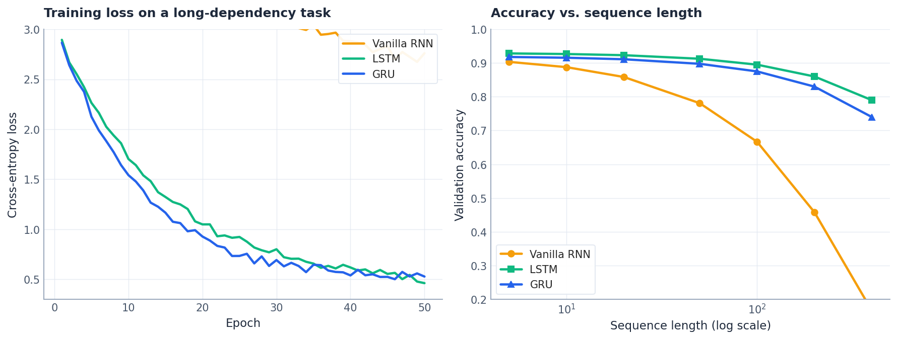
Loss curves and accuracy vs. sequence length, comparing RNN, LSTM, GRU

The two panels above tell the story qualitatively. On a long-dependency task, vanilla RNN training plateaus at a high loss while LSTM and GRU keep descending — the gradient highway is doing real work. As sequence length grows, vanilla RNN accuracy collapses, while LSTM and GRU degrade gracefully. The gap between LSTM and GRU is small in most settings, which is why GRU is a reasonable default.

Attention preview

The encoder squeezes everything into one vector $c$. For long sentences, this bottleneck loses information. Attention lets the decoder consult every encoder hidden state, with learned weights:

$$ \alpha_{tj} = \frac{\exp(\mathrm{score}(s_t, h_j))}{\sum_k \exp(\mathrm{score}(s_t, h_k))}, \qquad c_t = \sum_j \alpha_{tj}\, h_j. $$

The context vector becomes a time-varying weighted sum of encoder states. This was the bridge from RNNs to Transformers, which we cover in Part 4.

Common questions

Why tanh instead of ReLU in vanilla RNNs? Tanh outputs values in $[-1, 1]$, which keeps the hidden state bounded across time. ReLU has unbounded positive output, so a recurrent application can blow up exponentially. LSTMs use sigmoid for gates (a soft 0–1 switch) and tanh for candidates (zero-centred values that can both add and subtract from the cell state).

What is teacher forcing, and what is its downside? During training we feed the ground-truth previous token as the decoder input rather than the model’s own prediction. This stabilises learning early on but creates a train/test mismatch — at inference the decoder must consume its own (noisy) outputs, which it has never seen during training. A standard mitigation is scheduled sampling: gradually increase the probability of feeding the model’s own prediction as training progresses.

How does temperature affect generation? It rescales logits before softmax: $P(w) = \mathrm{softmax}(\text{logits}/T)$. Low $T$ (0.5) is peaky and conservative; high $T$ (1.5) is flat and creative but error-prone. Greedy decoding is the limit $T \to 0$.

Are RNNs still relevant after Transformers? Transformers dominate offline NLP benchmarks, but RNNs remain useful when you need (i) a small parameter budget, (ii) genuine streaming/online inference (no need to re-attend over the whole prefix), or (iii) constant memory per step regardless of sequence length. They also remain a common ingredient in time-series forecasting and on-device speech models. And because attention can be motivated as “what if we replaced the LSTM’s forget gate with a learned look-back over all previous states?”, understanding RNNs is the cleanest path to understanding Transformers.

Key takeaways

RNNs process sequences with memory via recurrent connections and parameter sharing — the same weights at every step.
Vanilla RNNs fail on long sequences because the chained Jacobian product $\prod \partial h_{k+1} / \partial h_k$ shrinks (or explodes) exponentially.
LSTMs add an additive cell-state highway gated by forget/input/output, giving gradients a path that does not vanish.
GRUs simplify LSTMs to two gates and one state, often matching LSTM accuracy with ~25% fewer parameters.
Bidirectional and stacked variants widen the per-position context and add depth, respectively.
Seq2Seq encoder-decoders map sequences to sequences but bottleneck on a single context vector $c$ — a limitation that motivates attention, the topic of Part 4.

Part	Topic	Link
1	Introduction and Text Preprocessing	<– Read
2	Word Embeddings and Language Models	<– Previous
3	RNN and Sequence Modeling (this article)
4	Attention Mechanism and Transformer	Read next –>
5	BERT and Pretrained Models	Read –>
6	GPT and Generative Models	Read –>

NLP Part 3: RNN and Sequence Modeling

What you will learn

2. The vanishing gradient problem

3. Long Short-Term Memory (LSTM)

The three gates

Why this fixes vanishing gradients

The conveyor-belt analogy

4. Gated Recurrent Unit (GRU)

LSTM vs. GRU

5. Bidirectional RNNs

6. Stacked RNNs

7. Sequence-to-sequence models

8. PyTorch implementation: character-level text generator

Dataset preparation

Model

Training loop

Sampling — temperature controls creativity

9. PyTorch implementation: a minimal Seq2Seq translator

Data and vocabulary

Encoder and decoder

Training (with teacher forcing)

Inference

10. How they actually compare

Attention preview

Common questions

Key takeaways

Series Navigation

Liked this piece?

What you will learn

1. The core idea: recurrence and parameter sharing

2. The vanishing gradient problem

3. Long Short-Term Memory (LSTM)

The three gates

Why this fixes vanishing gradients

The conveyor-belt analogy

4. Gated Recurrent Unit (GRU)

LSTM vs. GRU

5. Bidirectional RNNs

6. Stacked RNNs

7. Sequence-to-sequence models

8. PyTorch implementation: character-level text generator

Dataset preparation

Model

Training loop

Sampling — temperature controls creativity

9. PyTorch implementation: a minimal Seq2Seq translator

Data and vocabulary

Encoder and decoder

Training (with teacher forcing)

Inference

10. How they actually compare

Attention preview

Common questions

Key takeaways

Series Navigation

Liked this piece?