ODE Chapter 2: First-Order Methods

A bank account, a drug clearing the bloodstream, a tank of brine, a charging capacitor — they all obey the same kind of equation: a first-order ODE. The trick is recognising which of four shapes you are looking at, because each shape has a closed-form move that solves it cleanly. By the end of this chapter you will pattern-match an unfamiliar first-order equation in seconds and know exactly which lever to pull.

What you will learn

How to spot a separable equation and integrate it directly.
The integrating factor that turns a linear equation into a perfect derivative.
The exactness test and what it means geometrically: solutions are level curves of a potential.
The Bernoulli substitution $v = y^{1-n}$ that linearises a whole family of nonlinear equations.
Five real applications: drug half-life, RC charging, salt mixing, logistic growth, exponential interest — each one a small case study you can reuse.

Prerequisites

Chapter 1 ideas: what an ODE is, what an initial value problem is, how a slope field looks.
Standard integration: substitution, integration by parts, partial fractions.

1. Separable equations: the most natural form

1.1 The shape

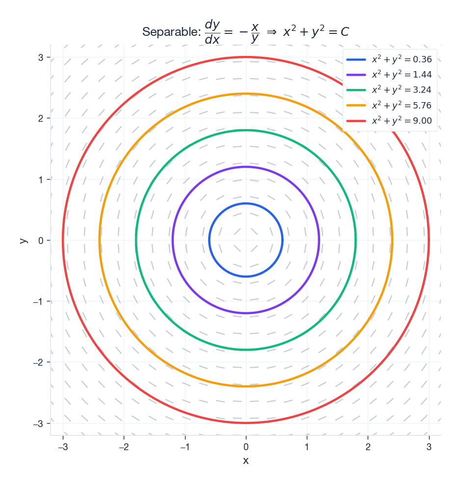
A first-order ODE is separable when the right-hand side factors into “something in $x$” times “something in $y$”:

$$ \frac{dy}{dx} \;=\; g(x)\,h(y). $$

That factorisation is exactly what lets us put all the $y$’s on one side and all the $x$’s on the other:

$$ \frac{dy}{h(y)} \;=\; g(x)\,dx \qquad\Longrightarrow\qquad \int \frac{dy}{h(y)} \;=\; \int g(x)\,dx + C. $$

The constant $C$ is the family parameter — every choice picks out one solution curve. In the figure below, separating $\frac{dy}{dx} = -x/y$ gives $y\,dy + x\,dx = 0$, which integrates to $x^2 + y^2 = C$: a one-parameter family of circles. The slope-field arrows are tangent to these circles everywhere — exactly what “solution” means.

Solution curves of dy/dx = -x/y are concentric circles, tangent to the slope field everywhere.

Separation collapses a 2-D slope field into a 1-D family of curves $x^2+y^2=C$.

1.2 Worked example: exponential growth and decay

Solve $\dfrac{dy}{dx} = ky$ for constant $k$.

Separate. $\;\dfrac{dy}{y} = k\,dx$.
Integrate both sides. $\;\ln|y| = kx + C_1$.
Exponentiate. $\;y = A e^{kx}$, where $A = \pm e^{C_1}$ absorbs the sign and the constant.

What just happened? The growth rate $k$ controls the time scale, not the shape. Two interpretations:

$k > 0$: doubling every $\ln 2 / k$ — populations with no resource limit, continuously compounded interest, runaway nuclear chain reaction.
$k < 0$: half-life of $\ln 2 / |k|$ — radioactive decay, a charged capacitor draining, a drug being cleared by the liver.

1.3 Application: drug metabolism and the half-life rule

Most drugs follow first-order elimination: the rate at which they leave the bloodstream is proportional to how much is in there:

$$ \frac{dC}{dt} = -kC, \qquad C(t) = C_0 e^{-kt}. $$

The half-life $t_{1/2}$ is the time for $C$ to fall to $C_0/2$. Setting $C_0/2 = C_0 e^{-k t_{1/2}}$ and solving gives the universal formula

$$ t_{1/2} = \frac{\ln 2}{k} \approx \frac{0.693}{k}. $$

For ibuprofen $t_{1/2} \approx 2$ h. Starting from a 400 mg dose:

Time	Remaining	What it means
0 h	400 mg	peak
2 h	200 mg	one half-life
4 h	100 mg	two half-lives
6 h	50 mg	sub-therapeutic

That’s why ibuprofen is dosed every 4–6 h: any longer and the level falls below the therapeutic window; any shorter and it accumulates. The “5 half-lives to clear” rule of thumb (about 99% gone) drops out of the same equation.

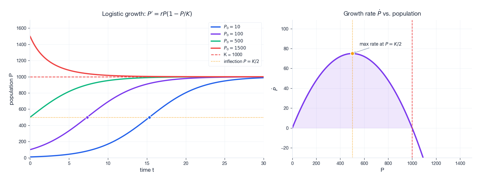
1.4 Application: the logistic equation

Pure exponential growth $P' = rP$ is a fantasy: nothing grows forever. Verhulst (1838) added a brake — a carrying capacity $K$ — and got the equation that still anchors mathematical ecology:

$$ \frac{dP}{dt} = r P\left(1 - \frac{P}{K}\right). $$

It is separable. Partial fractions on the left give

$$ \int \!\left(\frac{1}{P} + \frac{1/K}{1 - P/K}\right)\,dP \;=\; \int r\,dt, $$

and exponentiating produces the logistic curve

$$ P(t) \;=\; \frac{K}{1 + \left(\dfrac{K}{P_0} - 1\right)e^{-rt}}. $$

Three structural facts fall out of the equation itself, before you ever solve it:

$P \ll K$: the bracket is $\approx 1$, so growth is nearly exponential.
$P = K/2$: the right-hand side is $rK/4$, the maximum possible rate.
$P \to K$: the bracket tends to zero — population saturates.

The right-hand panel below visualises this: the growth rate $\dot P$ as a function of $P$ is a downward parabola with peak at $K/2$ and roots at $P=0$ and $P=K$.

Logistic curves for several initial populations and the parabolic growth-rate curve dP/dt versus P.

Left: every solution converges to $K$. Right: the growth rate $\dot P = rP(1-P/K)$ peaks exactly at $P=K/2$.

2. First-order linear equations: the integrating factor

2.1 Standard form

$$ \frac{dy}{dx} + P(x)\,y \;=\; Q(x). $$

This is the workhorse of applied math. Whenever a quantity changes in proportion to itself plus an external forcing term, you get this shape.

2.2 The trick

Multiply through by

$$ \mu(x) \;=\; e^{\int P(x)\,dx}, $$

the integrating factor. The product rule then collapses the left side into a single derivative:

$$ \frac{d}{dx}\bigl[\mu(x)\,y\bigr] \;=\; \mu(x)\,Q(x). $$

Integrate once and divide by $\mu$:

$$ \boxed{\,y(x) \;=\; \frac{1}{\mu(x)} \left[\int \mu(x)\,Q(x)\,dx + C\right].\,} $$

That’s the entire method. Why does it work? $\mu$ is engineered so that $\mu' = \mu P$, exactly what the product rule demands.

2.3 Worked example: $y' + 2xy = x$

Step	Computation	Result
1. Identify	$P = 2x$, $\;Q = x$	—
2. Integrating factor	$\mu = \exp\!\int 2x\,dx$	$\mu = e^{x^2}$
3. Multiply	LHS becomes $\frac{d}{dx}[e^{x^2}y]$	RHS $= x e^{x^2}$
4. Integrate	$\int x e^{x^2} dx = \tfrac12 e^{x^2}$	$e^{x^2}y = \tfrac12 e^{x^2} + C$
5. Solve	divide by $e^{x^2}$	$y = \tfrac12 + C e^{-x^2}$

As $x \to \pm\infty$ the term $C e^{-x^2}$ vanishes, so every solution funnels into the equilibrium $y = 1/2$. The constant of integration only matters in a transient near the origin.

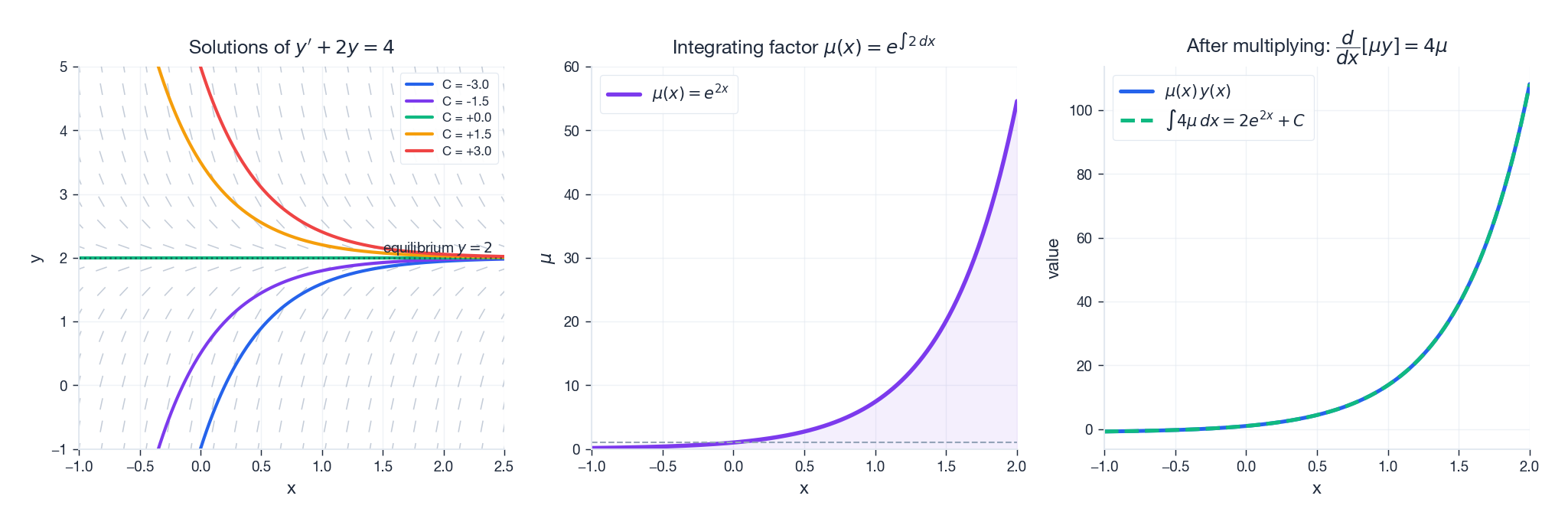
2.4 What the integrating factor does visually

Three side-by-side panels make it obvious. We pick $y' + 2y = 4$ (so $P = 2$, $\mu = e^{2x}$, equilibrium $y=2$).

Slope field with solution family for y’ + 2y = 4, the integrating factor e^{2x}, and the collapse of LHS into a perfect derivative.

Left: every solution $y = 2 + Ce^{-2x}$ rushes towards the equilibrium $y=2$. Middle: the integrating factor $e^{2x}$ is just a clean exponential. Right: after multiplying, $\mu(x)y(x)$ matches $\int 4\mu\,dx$ — the whole left side has become one antiderivative.

2.5 Application: charging an RC circuit

Kirchhoff’s voltage law on a series resistor $R$ and capacitor $C$ driven by source $V_s$ gives

$$ RC\,\frac{dV_c}{dt} + V_c \;=\; V_s. $$

Compare with the standard form: $P(t) = 1/RC$, $Q(t) = V_s/RC$. The integrating factor is $\mu(t) = e^{t/RC}$. With $V_c(0)=0$ this works out to

$$ V_c(t) \;=\; V_s\bigl(1 - e^{-t/\tau}\bigr), \qquad \tau = RC. $$

The time constant $\tau$ is what every electrical engineer memorises:

Time	$V_c/V_s$	Practical reading
$\tau$	63.2%	“one time constant”
$3\tau$	95.0%	usable as charged in most logic
$5\tau$	99.3%	considered “fully charged”

Same formula, with a sign flip and $V_s = 0$, governs discharging — and explains why your camera flash takes a noticeable second to recharge between shots.

3. Exact equations

3.1 The geometric idea

Write the ODE in the differential form

$$ M(x,y)\,dx + N(x,y)\,dy = 0. $$

Suppose there exists a “potential” $F(x,y)$ such that

$$ \frac{\partial F}{\partial x} = M, \qquad \frac{\partial F}{\partial y} = N. $$

Then $M\,dx + N\,dy$ is precisely the total differential $dF$, the equation $dF = 0$ says $F$ is constant along solutions, and the entire solution family is

$$ F(x,y) \;=\; C. $$

The solution curves are the level sets of $F$. That is the whole picture, and it is profound: solving the ODE has been replaced by recovering a scalar function whose contour map is the solution family.

3.2 The exactness test

A potential exists iff mixed partials match — that’s just $F_{xy} = F_{yx}$:

$$ \boxed{\,\dfrac{\partial M}{\partial y} \;=\; \dfrac{\partial N}{\partial x}.\,} $$

If this fails, the equation is not exact (yet — see §3.4).

3.3 Solving an exact equation, step by step

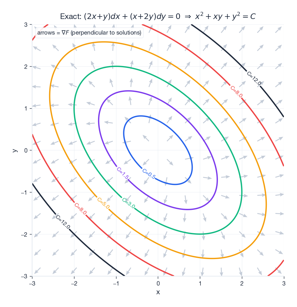
Take $(2x + y)\,dx + (x + 2y)\,dy = 0$. Check exactness: $M_y = 1 = N_x$. Good. Now reconstruct $F$:

Integrate $M$ with respect to $x$: $\;F = x^2 + xy + g(y)$.
Differentiate with respect to $y$ and match $N$: $\;x + g'(y) = x + 2y \Rightarrow g'(y) = 2y \Rightarrow g(y) = y^2$.
Therefore $F(x,y) = x^2 + xy + y^2$, and the solution family is $x^2 + xy + y^2 = C$.

Geometrically these are tilted ellipses. The figure below overlays the gradient field $\nabla F = (M, N)$ on the level curves; the gradient is everywhere perpendicular to the level set, which is the formal way of saying that $\nabla F$ tells you “uphill” while the solution curve stays at the same height.

Level curves of F(x,y) = x^2 + xy + y^2 with the gradient field overlaid, showing perpendicularity.

Each contour is one solution. The grey arrows point along $\nabla F$, perpendicular to the contour — that’s the geometric content of “$dF = 0$ along solutions”.

3.4 Salvage: making a non-exact equation exact

If $M_y \neq N_x$, multiply by $\mu(x,y)$ and look for a $\mu$ that fixes things. Two common cases admit closed forms:

Condition	Use
$(M_y - N_x)/N$ depends only on $x$	$\mu(x) = \exp\!\int \dfrac{M_y - N_x}{N}\,dx$
$(N_x - M_y)/M$ depends only on $y$	$\mu(y) = \exp\!\int \dfrac{N_x - M_y}{M}\,dy$

This is the same construction as the linear-equation integrating factor — in fact, the linear method is a special case of this one.

4. Bernoulli equations

4.1 The shape

$$ \frac{dy}{dx} + P(x)\,y \;=\; Q(x)\,y^{n}, \qquad n \neq 0, 1. $$

When $n = 0$ it’s already linear; when $n = 1$ it’s separable. The interesting range is everything else, where the $y^n$ term ruins linearity.

4.2 The substitution

Let $v = y^{1-n}$. Then $\dfrac{dv}{dx} = (1-n)\,y^{-n}\,\dfrac{dy}{dx}$. Multiply the original equation by $(1-n) y^{-n}$ and rewrite:

$$ \frac{dv}{dx} + (1-n)P(x)\,v \;=\; (1-n)Q(x). $$

That is linear in $v$. Solve it with the integrating factor of §2, then convert back via $y = v^{1/(1-n)}$.

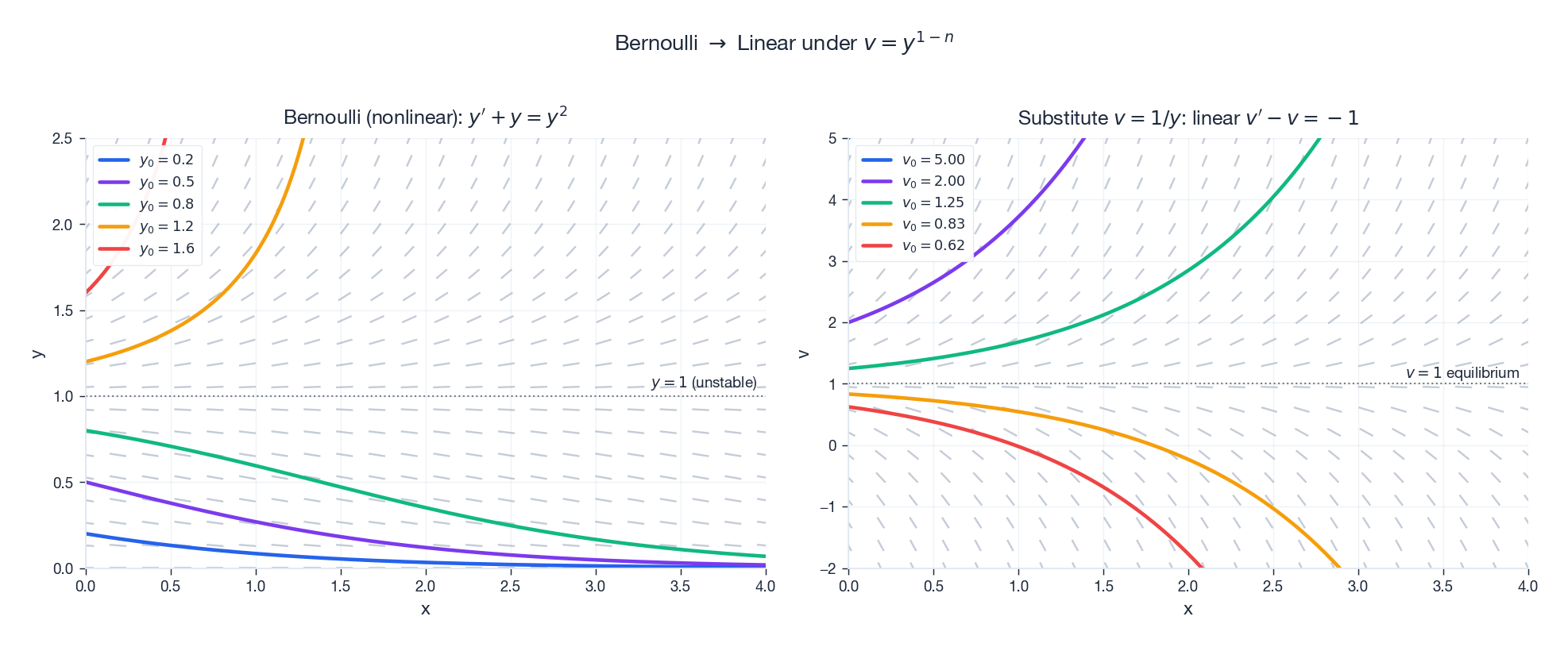
4.3 What the substitution does geometrically

Take $y' + y = y^2$ (so $n = 2$, $v = 1/y$). The substitution turns it into the linear equation $v' - v = -1$, whose solutions are exponentials around the equilibrium $v = 1$. In $v$-space the family is straight and orderly; in the original $y$-space it is curved and contains a finite-time blow-up.

Bernoulli y’ + y = y^2 in the original (x, y) plane and in the linearised (x, v) plane after the substitution v = 1/y.

The same five trajectories. Left in $(x, y)$: nonlinear, with the unstable equilibrium $y=1$. Right in $(x, v)$: linear, with the stable equilibrium $v=1$ that corresponds to $y=1$ from below.

The same substitution trick recovers the logistic equation: it is Bernoulli with $n = 2$, $P(t) = -r$, $Q(t) = -r/K$. So the messy partial-fraction integration of §1.4 is really just an integrating-factor calculation in disguise.

5. A worked application: salt in a tank

This is the classic “compartment model” — the same skeleton you will meet again in epidemiology, pharmacokinetics and chemical engineering.

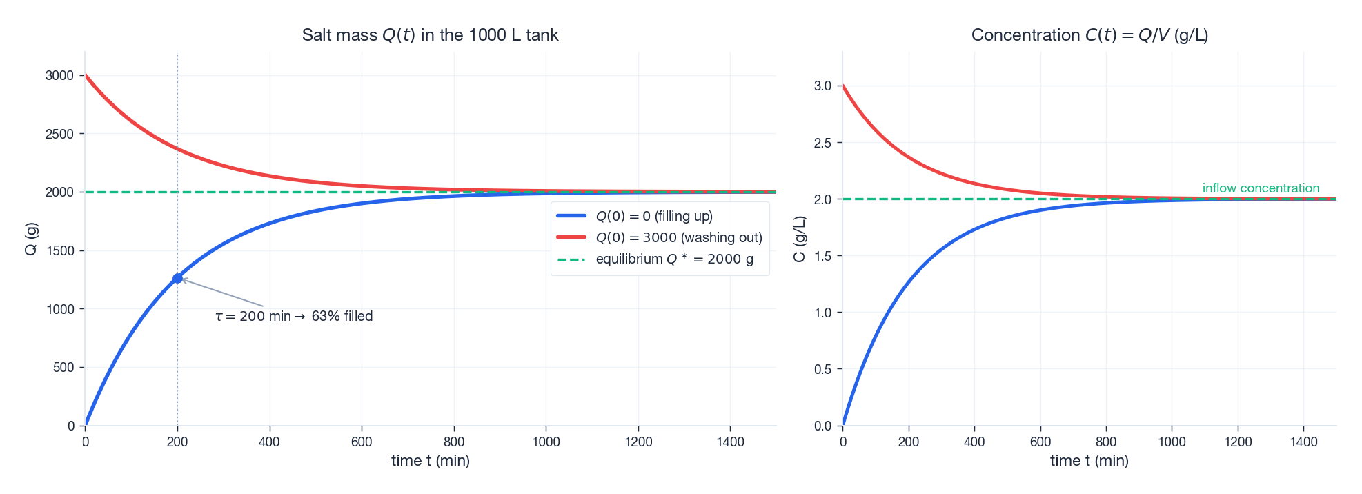
Setup. A 1000 L tank starts with pure water. Brine with concentration $2$ g/L flows in at $5$ L/min. The tank is well-stirred and drains at the same rate, so the volume stays constant. Find the salt mass $Q(t)$.

Model. Salt in minus salt out:

$$ \underbrace{\frac{dQ}{dt}}{\text{rate of change}} = \underbrace{5 \cdot 2}{\text{in: g/min}}

\underbrace{5 \cdot \tfrac{Q}{1000}}_{\text{out: g/min}} = 10 - \tfrac{Q}{200}, \qquad Q(0) = 0. $$

Solve. This is linear: $Q' + \tfrac{1}{200}Q = 10$. Integrating factor $\mu = e^{t/200}$ gives

$$ Q(t) \;=\; 2000\bigl(1 - e^{-t/200}\bigr). $$

Read the answer. The equilibrium is $Q^\ast = 2000$ g, i.e. concentration $2$ g/L — exactly the inflow concentration. The time constant $\tau = 200$ min controls how fast we get there. The same equation with $Q(0) > Q^\ast$ describes a salty tank being washed clean — the curves below show both regimes converging to the same equilibrium.

Salt mass Q(t) approaching 2000 g for two initial conditions, with concentration panel.

Two scenarios, one equilibrium. Filling up from $Q(0)=0$ and washing out from $Q(0)=3000$ both reach the inflow concentration $2$ g/L; only the sign of the deviation changes.

6. Numerical methods preview

Closed-form tricks fail the moment $f(x,y)$ is messy enough — and most real-world equations are. The answer is to step along the slope field.

6.1 Euler’s method

The simplest possible idea: replace the curve with its tangent on each step.

$$ y_{n+1} \;=\; y_n + h\,f(t_n, y_n). $$

Local truncation error per step: $O(h^2)$.
Global error after $1/h$ steps: $O(h)$. Hence “first-order method”.

Cheap, easy, often inadequate.

6.2 Runge–Kutta 4 (RK4)

The standard workhorse. Combine four slope evaluations per step:

$$ k_1 = f(t_n, y_n), \qquad k_2 = f\!\left(t_n + \tfrac{h}{2},\, y_n + \tfrac{h}{2}k_1\right), $$$$ k_3 = f\!\left(t_n + \tfrac{h}{2},\, y_n + \tfrac{h}{2}k_2\right), \qquad k_4 = f(t_n + h,\, y_n + h k_3), $$$$ y_{n+1} \;=\; y_n + \frac{h}{6}\bigl(k_1 + 2k_2 + 2k_3 + k_4\bigr). $$

Global error $O(h^4)$ — four orders of magnitude better than Euler at the same step size, for the cost of three extra evaluations.

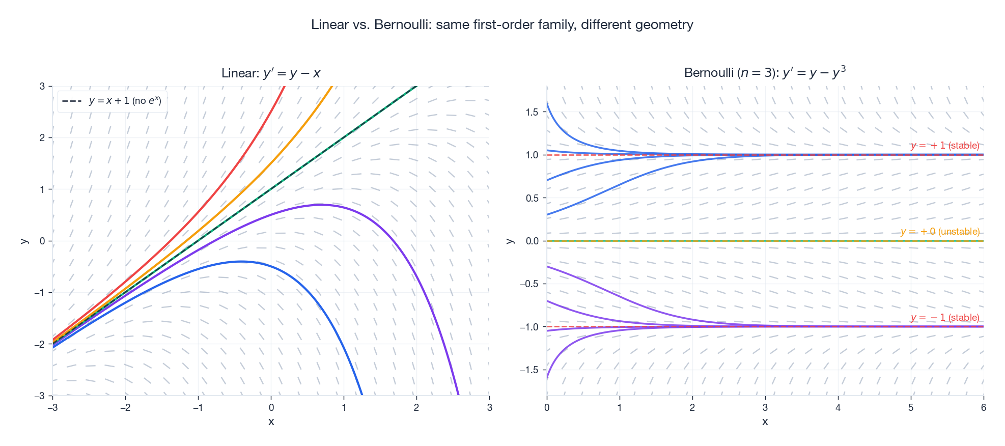
6.3 Slope fields tell you what the integrator will see

Before you reach for a numerical solver, look at the right-hand side. Two superficially similar equations can have radically different long-term behaviour:

Slope fields of a linear equation y’=y-x and the Bernoulli equation y’=y-y^3, with representative trajectories.

Linear (left): one straight-line solution $y=x+1$, all others diverge exponentially. Bernoulli (right): three equilibria at $y=-1, 0, +1$; trajectories are squeezed onto $\pm 1$ regardless of initial sign. Same first-order family, completely different geometry.

6.4 SciPy in three lines

Newton’s law of cooling: $T' = -k(T - T_{\text{env}})$ with $T(0) = 90$°C, $T_{\text{env}} = 20$°C, $k = 0.1$ /min.

 1
 2
 3
 4
 5
 6
 7
 8
 9
10
11
12
from scipy.integrate import solve_ivp
import numpy as np

def cooling(t, T, k=0.1, T_env=20):
    return -k * (T - T_env)

sol = solve_ivp(cooling, [0, 60], [90.0], method="RK45", dense_output=True)

t = np.linspace(0, 60, 300)
T = sol.sol(t)[0]
print(f"At t=10 min: {T[50]:.1f} C")
print(f"At t=30 min: {T[150]:.1f} C")

solve_ivp adapts the step size automatically. For most problems you do not need to write your own RK4; you need to know when the standard solver will struggle (stiff systems — see Chapter 11).

7. Summary: the four-question filter

When you meet a first-order equation, run it through these in order — the first “yes” tells you the method.

Question	If yes	Method
Can I write it as $y' = g(x)\,h(y)$?	Separable	Move terms, integrate both sides
Is it $y' + P(x)y = Q(x)$?	Linear	Integrating factor $\mu = e^{\int P\,dx}$
Is it $M\,dx + N\,dy = 0$ with $M_y = N_x$?	Exact	Reconstruct potential $F$; solution is $F = C$
Is it $y' + Py = Qy^n$ with $n \notin \{0,1\}$?	Bernoulli	Substitute $v = y^{1-n}$, then go to row 2
None of the above?	—	Numerical methods (Chapter 11) or look for a clever substitution

The four methods are not independent. The integrating factor for a linear equation is the special case of the integrating factor that fixes a non-exact equation. The Bernoulli substitution reduces nonlinear to linear. So learning these four well is really learning one idea — find the change of variable that turns the equation into something that integrates by inspection — applied four ways.

8. Exercises

Basic.

Solve $y' = y^2 \sin x$ with $y(0) = 1$. Where does the solution blow up?
Solve $y' + y = e^{-x}$. Identify the transient and steady-state parts.
Verify that $(2xy + 3)\,dx + (x^2 + 1)\,dy = 0$ is exact and solve it.
A 1000 L tank holds 50 kg of dissolved salt. Pure water enters at 10 L/min; the well-mixed solution leaves at the same rate. Find $Q(t)$ and the time to halve the salt mass.

Advanced.

Solve the Bernoulli equation $y' + y = y^3$. Sketch the phase line and identify the equilibria.
For $y' = 3y^{2/3}$ with $y(0) = 0$, exhibit at least two distinct solutions on $[0, \infty)$. Why does this not contradict the existence-uniqueness theorem?
A bacterial population obeys $P' = 0.5\,P(1 - P/1000)$ with $P(0) = 50$. Find $P(t)$ explicitly and compute the time at which the growth rate is maximal.

Programming.

Implement Euler and RK4 from scratch. Compare their global error on $y' = -y$, $y(0) = 1$ over $[0, 5]$ at step sizes $h = 0.5, 0.1, 0.01$. Plot $\log(\text{error})$ versus $\log(h)$ and verify the predicted slopes 1 and 4.
Reproduce the slope-field comparison of §6.3 yourself: use numpy.meshgrid and matplotlib.pyplot.quiver for the field, then scipy.integrate.solve_ivp for the trajectories. Try $y' = y - y^5$ and identify the equilibria.

References

Boyce & DiPrima, Elementary Differential Equations and Boundary Value Problems, Wiley (2012). The standard undergraduate reference; Chapters 2–3 cover everything above with classical rigour.
Zill, A First Course in Differential Equations with Modeling Applications, Cengage (2017). Heavier on applications; the mixing and circuit examples are particularly clean.
Strogatz, Nonlinear Dynamics and Chaos, Westview (2014). Chapter 2’s phase-line treatment of the logistic equation is essential reading after this chapter.
SciPy documentation: scipy.integrate . The reference for solve_ivp, including its choice of methods (RK45, Radau, BDF) and event handling.

Series Navigation