Ordinary Differential Equations (8): Nonlinear Systems and Phase Portraits
Step beyond linearity: predator-prey oscillations, competition exclusion, Van der Pol limit cycles, Hamiltonian systems, and the Poincaré-Bendixson theorem -- the full toolkit for nonlinear 2D dynamics.
The real world is nonlinear. Predator-prey cycles, heartbeat rhythms, neuron firing — none of these can be captured by linear equations. When superposition fails, the world acquires new behaviors: limit cycles, multiple equilibria, bistability, hysteresis. This chapter gives you the geometric and analytic tools to read those behaviors directly off a 2D phase portrait.
What You Will Learn#
- Why nonlinear systems are fundamentally different from linear ones
- Lyapunov stability visualized: level sets, bowls, and basins
- Linearization vs. the full nonlinear picture (Hartman-Grobman in action)
- Lotka-Volterra predator-prey: closed orbits and conserved quantities
- Competition models: four canonical outcomes
- Van der Pol oscillator and the geometry of limit cycles
- Gradient and Hamiltonian systems
- Poincaré-Bendixson: why 2D systems cannot be chaotic
Prerequisites#
- Chapter 6 : linear systems, phase portrait classification
- Chapter 7 : stability, linearization, Lyapunov functions
From Linear to Nonlinear#
Linear systems obey superposition: if $\mathbf{x}_1$ and $\mathbf{x}_2$ are solutions, so is $c_1\mathbf{x}_1 + c_2\mathbf{x}_2$ . This is the engine that powers the entire toolkit of Chapters 1-6 — exponential ansatz, eigenvectors, fundamental matrices.
Nonlinear systems break this rule and pay the price — closed-form solutions vanish. But they get something priceless in return:
- Multiple equilibria, each with its own stability type
- Limit cycles — isolated, stable periodic orbits (impossible in linear systems)
- Bistability and hysteresis — memory of initial conditions
- Sensitive dependence — chaos, in 3D and beyond (Chapter 9 )
Almost every interesting system in physics, biology, chemistry, neuroscience, and economics is nonlinear.
Lyapunov Stability, Visualized#
A Lyapunov function $V(\mathbf{x})$ is a scalar that decreases along trajectories ($\dot V \leq 0$ ). Geometrically, level sets of $V$ form a nested family of “bowls” around the equilibrium, and trajectories cross them inward.
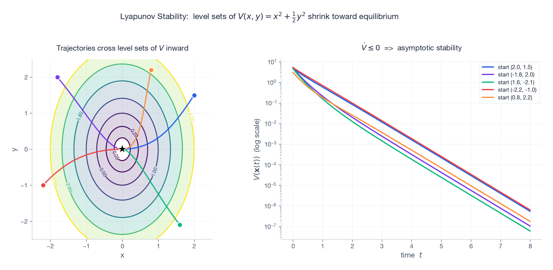
Once you see Lyapunov stability as “trajectories falling down a bowl”, every theorem becomes obvious:
- $\dot V \leq 0$ : trajectories never go uphill -> they stay in the smallest bowl that contains the start (stability).
- $\dot V < 0$ strictly: they keep falling -> they reach the bottom (asymptotic stability).
- $\dot V > 0$ : trajectories climb out -> instability.
LaSalle generalizes: when $\dot V$ vanishes on a set, trajectories settle on the largest invariant subset of that set.
Phase Portraits and Nullclines#
For $x' = f(x,y),\ y' = g(x,y)$ :
- The $x$ -nullcline is the curve $f(x,y) = 0$ . There $\dot x = 0$ , so trajectories cross it vertically.
- The $y$ -nullcline is the curve $g(x,y) = 0$ . Trajectories cross it horizontally.
- Equilibria sit at intersections of the two nullclines.
- The signs of $f$ and $g$ in each region tell you the direction of flow.
Nullcline analysis is the cheapest way to sketch a phase portrait by hand.
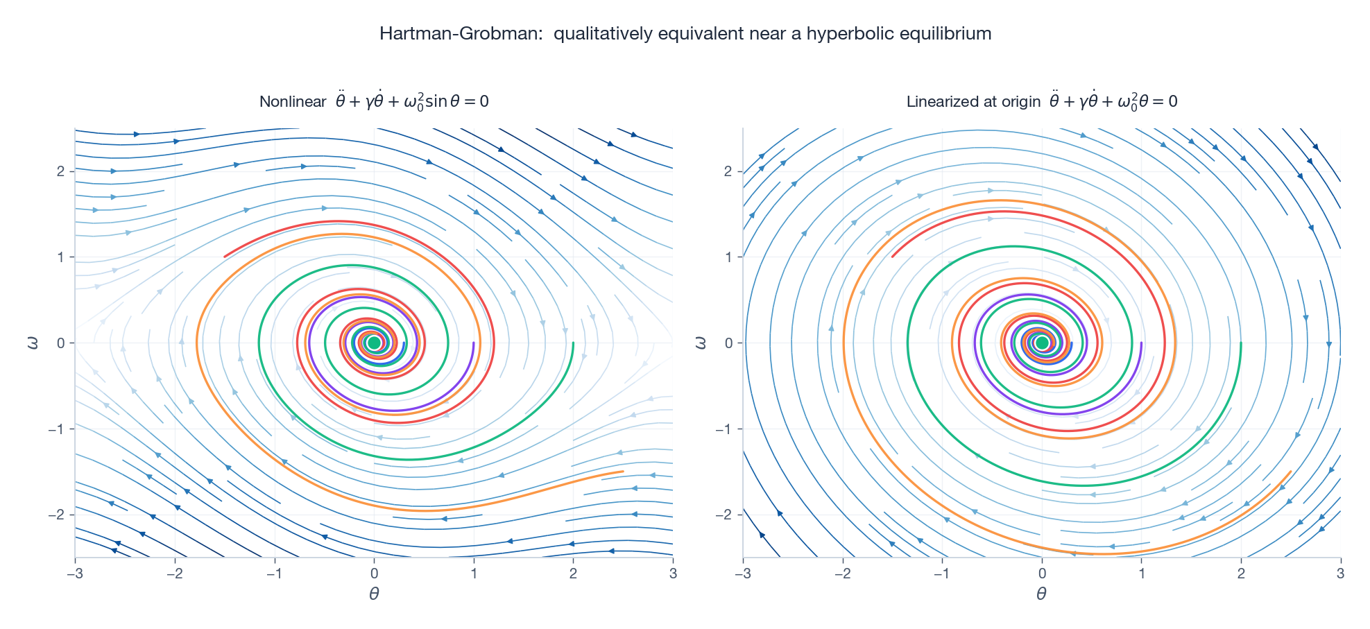
Linearization: Local Truth, Global Surprise#
Near a hyperbolic equilibrium, the Jacobian’s eigenvalues completely determine the local picture (Hartman-Grobman). But far from the equilibrium, all bets are off. The damped pendulum makes this dramatic:
| Linear-eigenvalue type | Local equilibrium | Stability (nonlinear) |
|---|---|---|
| $\lambda_1 < \lambda_2 < 0$ (real) | Stable node | Asymptotically stable |
| $0 < \lambda_1 < \lambda_2$ (real) | Unstable node | Unstable |
| $\lambda_1 < 0 < \lambda_2$ | Saddle | Unstable |
| $\alpha \pm \beta i,\ \alpha < 0$ | Stable spiral | Asymptotically stable |
| $\alpha \pm \beta i,\ \alpha > 0$ | Unstable spiral | Unstable |
| $\pm \beta i$ | Center | Inconclusive — nonlinear terms decide |
| |
Lotka-Volterra Predator-Prey#
The model#
$$x' = \alpha x - \beta xy, \qquad y' = \delta xy - \gamma y$$- $x$ : prey population, $y$ : predator population
- Trivial equilibrium $(0,0)$ : saddle
- Coexistence equilibrium $(\gamma/\delta,\ \alpha/\beta)$ : Jacobian eigenvalues $\pm i\sqrt{\alpha\gamma}$ (a center)
makes every orbit closed. Time-series and phase-plane look like this:
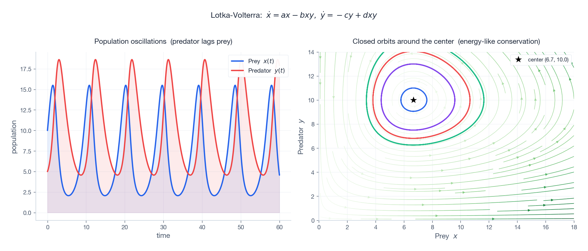
The cycle in words#
- Abundant prey -> predators thrive -> predator population rises.
- Many predators -> prey depleted -> prey crashes.
- Few prey -> predators starve -> predator population falls.
- Few predators -> prey rebounds -> back to step 1.
Limitations#
- Structurally unstable. The slightest extra term destroys the closed orbits.
- No carrying capacity. Prey grow unbounded if predators are absent.
- Ignores space and time delays.
These flaws drove the development of the more realistic models in the next section.
Competition Model: Four Outcomes#
$$\begin{aligned} x' &= r_1 x\!\left(1 - \frac{x + \alpha_{12}y}{K_1}\right), \\ y' &= r_2 y\!\left(1 - \frac{y + \alpha_{21}x}{K_2}\right). \end{aligned}$$The product $\alpha_{12}\,\alpha_{21}$ — the strength of mutual interference — determines which of four pictures you get.
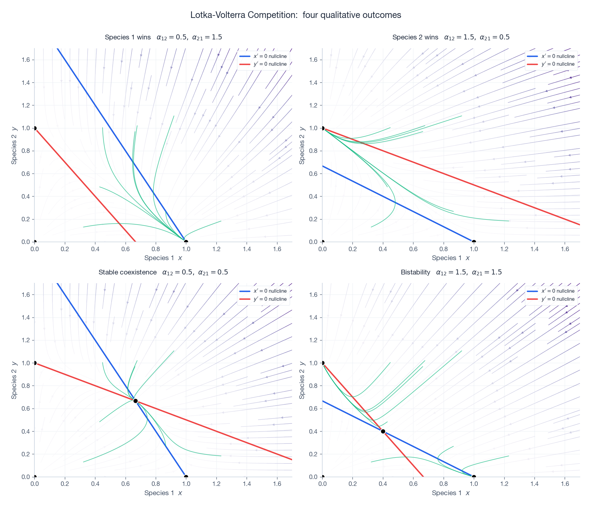
| Regime | Condition | Outcome |
|---|---|---|
| Weak interference | $\alpha_{12} < 1,\ \alpha_{21} < 1$ | Stable coexistence |
| Strong interference | $\alpha_{12} > 1,\ \alpha_{21} > 1$ | Bistability — winner depends on starting populations |
| Asymmetric | $\alpha_{12} < 1,\ \alpha_{21} > 1$ | Species 1 wins |
| Asymmetric | $\alpha_{12} > 1,\ \alpha_{21} < 1$ | Species 2 wins |
This is competitive exclusion in mathematical clothing.
Van der Pol: Limit Cycles from Nonlinear Damping#
$$x'' - \mu(1 - x^2)x' + x = 0$$The genius is in the damping coefficient $-\mu(1 - x^2)$ :
- Inside $|x| < 1$ : damping is negative — the system pumps energy in.
- Outside $|x| > 1$ : damping is positive — energy bleeds out.
Trajectories from inside grow, trajectories from outside shrink, and both settle on a single stable limit cycle — an isolated periodic orbit that attracts everything in its basin.
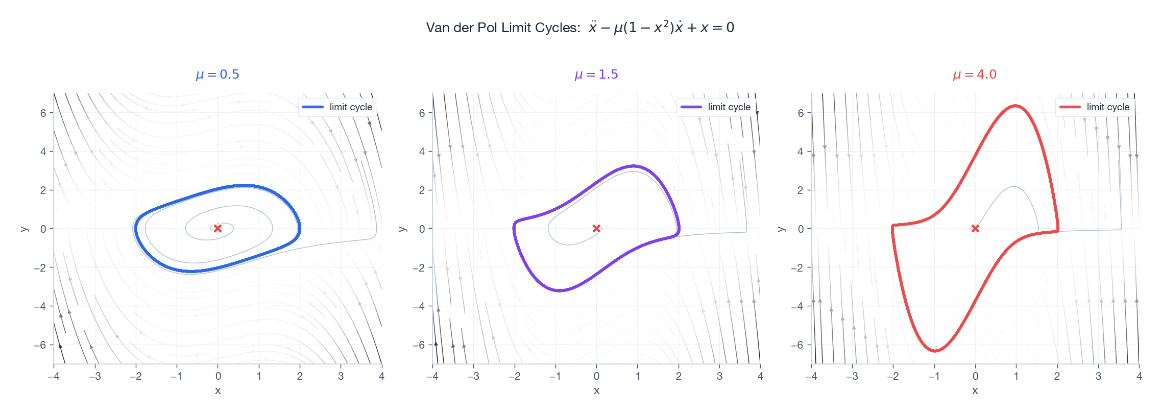
Where this shows up: heartbeat pacemaker cells, neuron action potentials, electronic oscillator circuits, geyser eruptions, business cycles.
Gradient and Hamiltonian Systems: Two Special Worlds#
Gradient systems: $\mathbf{x}' = -\nabla V$ #
- Trajectories follow the steepest descent of $V$ .
- $\dot V = -|\nabla V|^2 \leq 0$ — the potential always decreases.
- No periodic orbits possible (you can’t go around a hill and end up lower).
- Machine learning’s gradient descent is the discrete cousin.
Hamiltonian systems: $x' = \dfrac{\partial H}{\partial y},\ y' = -\dfrac{\partial H}{\partial x}$ #
- $H$ is conserved along every trajectory ($\dot H = 0$ ).
- Phase-space volume is preserved (Liouville’s theorem).
- Orbits are level curves of $H$ .
- The undamped pendulum is a textbook example.
These two worlds sit at opposite extremes of the dissipation spectrum.
Poincaré-Bendixson: 2D Cannot Be Chaotic#
Theorem (Poincaré-Bendixson). A bounded trajectory of a smooth 2D continuous system that does not approach any equilibrium must converge to a closed orbit.
In words: in 2D, the only long-term behaviors are equilibrium or periodic. There is no room for chaos.
The Jordan curve theorem is the secret here — a closed orbit divides the plane in two, trapping the trajectory. Add a third dimension and the trajectory can escape over the orbit, opening the door to chaos (Chapter 9 ).
Bendixson’s criterion (no closed orbits). If $\partial f/\partial x + \partial g/\partial y$ has constant non-zero sign in a simply-connected region, no closed orbit lies inside it.
Numerical Methods Quick Reference#
| Method | Order | Notes |
|---|---|---|
| Euler | $O(h)$ | Simple but inaccurate |
| Improved Euler (Heun) | $O(h^2)$ | Average of two slopes |
| RK4 | $O(h^4)$ | Best accuracy/cost ratio |
| RK45 (Dormand-Prince) | adaptive | Default in scipy.integrate.solve_ivp |
| |
Exercises#
Conceptual.
- Why does superposition fail for $y' = y^2$ ? Give a concrete counterexample.
- Why are 2D continuous systems forbidden from being chaotic?
- Sketch by hand the phase portrait of $x' = y,\ y' = -x + x^3 - 0.2y$ (Duffing).
Computational.
- For $x' = x - x^3,\ y' = -y$ : find every equilibrium and classify each.
- Prove $V = x^2 + y^2$ is a Lyapunov function for $x' = -x + y^2,\ y' = -y$ .
- Verify $H = \delta x - \gamma\ln x + \beta y - \alpha\ln y$ is conserved for Lotka-Volterra.
Programming.
- Reproduce the four competition regimes in fig 5 and shade each basin of attraction.
- Numerically estimate the Van der Pol period $T(\mu)$ for $\mu \in \{0.1, 0.5, 1, 3, 10\}$ .
- Compare Euler vs. RK4 accuracy for the Van der Pol equation — find the $\mu$ at which Euler breaks down.
Limit Cycle Stability via Floquet Multipliers#
Equilibria are judged by Jacobian eigenvalues. Limit cycles $\gamma(t)$ are judged by Floquet multipliers — the answer to “if I nudge a trajectory sideways, how much is the nudge amplified after one period?”.
$$ \dot\delta = J\!\bigl(\gamma(t)\bigr)\,\delta. $$Integrate over one period to get the monodromy matrix $\Phi(T)$ . Its eigenvalues $\mu_i$ are the Floquet multipliers. One is forced to be $\mu_1 = 1$ (sliding along the orbit is just a phase shift); the rest decide stability:
- All other $|\mu_i| < 1$ → stable limit cycle (attracting).
- Any $|\mu_i| > 1$ → unstable.
Numerically you co-integrate the cycle and a fundamental matrix:
| |
Van der Pol with $\mu = 1$ : the non-trivial multiplier is about $0.04$ . Strongly attracting — trajectories visibly snap onto the cycle in a couple of revolutions.
Numerical Pitfalls That Bite#
Pitfall 1: Stiff system, explicit method. Lotka-Volterra is fine. Tweak it to $\dot x = -1000(x - \cos t) - \sin t$
and explicit RK4 needs $h < 2/1000$
for stability — 500 steps per second of simulation. Switch to LSODA or BDF. Diagnostic: Jacobian eigenvalues straddle several decades.
Pitfall 2: Hamiltonian system, non-symplectic integrator. The pendulum has $H = p^2/2 - \cos q$ . RK4 over $10^4$ steps shows visible energy drift. Leapfrog or symplectic Euler oscillates around the true energy without drift. This is the motivation for the symplectic networks chapter in the PDE-ML series.
Pitfall 3: Phase drift on long integrations. On a limit cycle or quasi-periodic orbit, classical methods accumulate linear phase error. Want a clean phase portrait after $10^4$ periods? Standard RK4 will not deliver. Use a geometric integrator with a moderately large step.
ML Connection: A Neural ODE Is a Phase Portrait#
A Neural ODE $\dot z = f_\theta(z, t)$ casts classification as “flow each input to the right region”. The phase portrait of the trained $f_\theta$ literally is the network behaviour:
- Topological obstructions are real. Dupont et al. (2019) showed Neural ODEs cannot learn a mapping that requires two disjoint curves to cross — ODE flows are homeomorphisms. Fix: augment the state space to $\mathbb{R}^{d+k}$ (ANODE). Direct consequence of phase-plane theory.
- Attractor pictures are interpretability. After training a 2D Neural ODE classifier, draw the vector field of $f_\theta$ . You see decision boundaries built from fixed points and stable manifolds, no SHAP needed.
- Stability regularisation. Adding $\|J_\theta\|_F^2$ to the loss bounds local stretching of the flow. It is an implicit adversarial robustness device that comes from this chapter, not from ML folklore.
Summary#
| Concept | Key Point |
|---|---|
| Nonlinearity | Superposition fails; richer dynamics |
| Lyapunov visualization | Trajectories cross level sets inward |
| Linearization | Locally accurate near hyperbolic equilibria; globally only suggestive |
| Lotka-Volterra | Closed orbits from a conserved quantity |
| Competition | Four outcomes via nullcline geometry |
| Van der Pol | Limit cycle from sign-changing damping |
| Gradient systems | No periodic orbits |
| Hamiltonian systems | Energy conserved; orbits are level curves |
| Poincaré-Bendixson | 2D rules out chaos |
References#
- Strogatz, Nonlinear Dynamics and Chaos, Westview Press (2015)
- Murray, Mathematical Biology I, Springer (2002)
- Hirsch, Smale, & Devaney, Differential Equations, Dynamical Systems, and Chaos, Academic Press (2012)
- Verhulst, Nonlinear Differential Equations and Dynamical Systems, Springer (1996)
This is Part 8 of the 18-part series on Ordinary Differential Equations.
- Part 1: Origins and Intuition
- Part 2: First-Order Methods
- Part 3: Higher-Order Linear Theory
- Part 4: The Laplace Transform
- Part 5: Power Series and Special Functions
- Part 6: Linear Systems and the Matrix Exponential
- Part 7: Stability Theory
- Part 8: Nonlinear Systems and Phase Portraits (current)
- Part 9: Chaos Theory and the Lorenz System
- Part 10: Bifurcation Theory
- Part 11: Numerical Methods
- Part 12: Boundary Value Problems
- Part 13: Introduction to PDEs
- Part 14: Epidemic Models
- Part 15: Population Dynamics
- Part 16: Fundamentals of Control Theory
- Part 17: Physics and Engineering Applications
- Part 18: Frontiers and Series Finale
ODE Foundations 18 parts
- 01 Ordinary Differential Equations (1): Origins and Intuition
- 02 Ordinary Differential Equations (2): First-Order Methods
- 03 Ordinary Differential Equations (3): Higher-Order Linear Theory
- 04 Ordinary Differential Equations (4): The Laplace Transform
- 05 Ordinary Differential Equations (5): Power Series and Special Functions
- 06 Ordinary Differential Equations (6): Linear Systems and the Matrix Exponential
- 07 Ordinary Differential Equations (7): Stability Theory
- 08 Ordinary Differential Equations (8): Nonlinear Systems and Phase Portraits you are here
- 09 Ordinary Differential Equations (9): Chaos Theory and the Lorenz System
- 10 Ordinary Differential Equations (10): Bifurcation Theory
- 11 Ordinary Differential Equations (11): Numerical Methods
- 12 Ordinary Differential Equations (12): Boundary Value Problems
- 13 Ordinary Differential Equations (13): Introduction to Partial Differential Equations
- 14 Ordinary Differential Equations (14): Epidemic Models and Epidemiology
- 15 Ordinary Differential Equations (15): Population Dynamics
- 16 Ordinary Differential Equations (16): Fundamentals of Control Theory
- 17 Ordinary Differential Equations (17): Physics and Engineering Applications
- 18 Ordinary Differential Equations (18): Frontiers and Series Finale