
Ordinary Differential Equations (11): Numerical Methods
From Euler's tangent step to Dormand-Prince adaptive integrators: a working numerics toolkit. Convergence orders, A-stability, stiffness, and when to reach for Radau or BDF instead of RK45.
Almost every interesting differential equation in science and engineering resists a closed-form solution. Nonlinear vector fields, variable coefficients, and thousands of coupled state variables — pen and paper fail long before the problem does. Numerical integration is the key. This chapter builds, evaluates, and compares a small set of algorithms that can solve almost any ODE you’ll encounter and provides diagnostics to spot when an integrator is misleading you.

What You Will Learn#
- The geometric idea behind Euler’s method, and why it costs you accuracy that classical Runge-Kutta gives back essentially for free
- A clean derivation of the order of accuracy and what “convergence rate$\mathcal{O}(h^p)$ ” really means in a log-log plot
- Adaptive step-size control via embedded RK methods (the engine inside
scipy.integrate.solve_ivp) - Stiffness: what it is, how to spot it, why explicit methods catastrophically fail, and how implicit methods (BDF, Radau) save the day
- Linear stability regions in the complex plane and what they tell you about choosing $h$
- A short tour of multistep methods, symplectic integrators for Hamiltonian flows, and a checklist for production use
Prerequisites: basic ODE concepts from Chapters 1-4 . Some Taylor-series fluency.
Why we need numerical methods#
The analytical methods of earlier chapters — separation of variables, integrating factors, Laplace transforms, eigenvalue expansions — are powerful but fragile. They work for narrow classes of equations and break the moment a real problem stops being symbolic-friendly. Take$\frac{dy}{dx} = \sin(xy).$ No closed form exists. The Navier-Stokes equations, the three-body problem, every chemical reaction network with more than a handful of species, the Lorenz system — all defeat symbolic methods. We have to settle for discrete approximations$y_n \approx y(x_n)$ at a sequence of grid points$x_n = x_0 + nh$ .
The questions are then:
- How do we choose the update rule$y_{n+1} = \Phi(y_n, h, f, \ldots)$ ?
- How does the error scale with$h$ ?
- How does the method behave when the equation is “stiff” — when small$h$ is required for stability rather than for accuracy?
We answer all three.
Forward Euler: the geometric idea#
Given$\dot{y} = f(x, y),\;y(x_0) = y_0$ , the simplest step replaces the curve by its tangent line:$y_{n+1} = y_n + h\,f(x_n, y_n).$ This is forward Euler, and it is the prototype of every explicit one-step scheme. The intuition: at every step you read the slope at your current location, walk a small distance$h$ in that direction, then re-read the slope. Like navigating a hillside in fog by always trusting the local incline.
Order of accuracy#
Taylor-expand the true solution:$y(x_n + h) = y(x_n) + h\,y'(x_n) + \tfrac{h^2}{2}y''(x_n) + \mathcal{O}(h^3).$ Subtracting the Euler step$y_{n+1} = y_n + h f(x_n, y_n)$ leaves a local truncation error of$\mathcal{O}(h^2)$ per step. Over a fixed interval$[x_0, X]$ we take$N = (X - x_0)/h$ steps, so the global error is$\mathcal{O}(h)$ . Halving the step size halves the error — a slow rate of return for the doubled cost.
Linear stability#
Apply Euler to the test equation$\dot{y} = \lambda y$ , $\mathrm{Re}\,\lambda < 0$ :$y_{n+1} = (1 + h\lambda)\,y_n.$ The amplification factor is$R(z) := 1 + z$ , where$z = h\lambda$ . Stability requires$|R(z)| \le 1$ . For real negative$\lambda$ , this forces$h < 2/|\lambda|$ . For oscillatory$\lambda$ on the imaginary axis, no$h>0$ is stable. Euler is conditionally stable at best, and useless for purely oscillatory problems.
| |
Heun, midpoint, and the Runge-Kutta family#
The cure for Euler’s first-order accuracy is to evaluate the slope more than once per step and combine the evaluations cleverly. The general structure of an explicit$s$ -stage Runge-Kutta method:$k_i = f\bigl(x_n + c_i h,\; y_n + h \textstyle\sum_{j<i} a_{ij}\,k_j\bigr), \quad y_{n+1} = y_n + h\sum_i b_i\,k_i.$ The coefficients$\{a_{ij}, b_i, c_i\}$ are arranged in a Butcher tableau.
Heun (improved Euler), order 2#
A predict-and-correct two-stage method:
- predictor: $\tilde y = y_n + h\,f(x_n, y_n)$
- corrector: $y_{n+1} = y_n + \tfrac{h}{2}\bigl[f(x_n, y_n) + f(x_n + h, \tilde y)\bigr]$
Local error$\mathcal{O}(h^3)$ , global error$\mathcal{O}(h^2)$ . Halve$h$ , cut the error to a quarter. Already much better.
Classical RK4, order 4#
$$k_1 = f(x_n, y_n)$$ $$k_2 = f\!\left(x_n + \tfrac{h}{2},\; y_n + \tfrac{h}{2}k_1\right)$$ $$k_3 = f\!\left(x_n + \tfrac{h}{2},\; y_n + \tfrac{h}{2}k_2\right)$$ $$k_4 = f(x_n + h,\; y_n + h k_3)$$ $$y_{n+1} = y_n + \tfrac{h}{6}(k_1 + 2k_2 + 2k_3 + k_4)$$The weights$(1, 2, 2, 1)/6$ mirror Simpson’s rule for integration; that is not a coincidence. Global error$\mathcal{O}(h^4)$ , four function evaluations per step, one of the great practical bargains in scientific computing. For non-stiff problems with smooth right-hand sides, this single algorithm has been the engineering default for over a century.
| |
Side-by-side: Euler vs RK4#
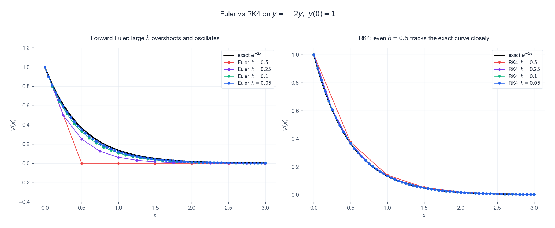
This is not a small effect. Going from order 1 to order 4 means the error budget at fixed$h$ is squared twice. To match RK4’s accuracy at$h=0.1$ with Euler, you would need$h \approx 10^{-5}$ — a hundred-thousand-fold cost.
Convergence orders, made visible#
The cleanest way to detect a method’s order is to compute the global error at the endpoint for a sequence of step sizes and plot it on log-log axes. The slope indicates the order.

Two practical lessons:
- The order is a hard speed limit. No amount of tuning will give you better than$\mathcal{O}(h^p)$ convergence from a method of order$p$ . To go faster, you need a higher-order method or extrapolation.
- The floor is real. RK4 at$h = 10^{-3}$ on a smooth problem already grazes machine precision. Below that, errors grow as round-off accumulates over more steps. Lowering$h$ past this floor hurts.
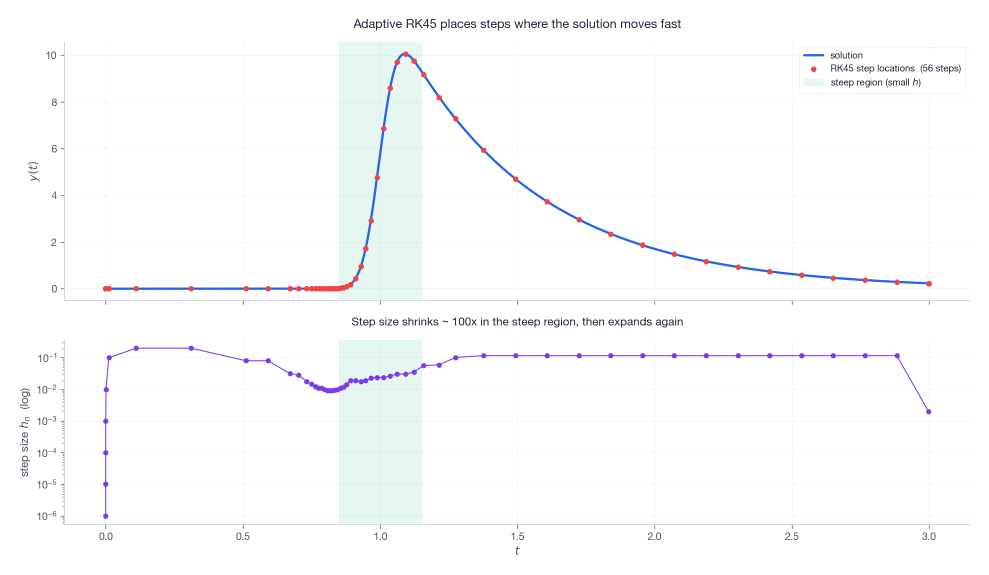
Adaptive step-size control#
Real solutions are not uniformly smooth. They have plateaus, sharp transients, slow tails. A fixed$h$ is either wastefully small on the plateau or dangerously large on the transient. The fix is adaptive stepping: choose$h$ on the fly to hold the local error near a user-specified tolerance.
The standard mechanism is embedded Runge-Kutta. Two methods of orders$p$
and$p+1$
share their stage evaluations. Their difference is an estimate of the local error$E_n$
. If$E_n > \text{tol}$
we reject the step and try a smaller$h$
; otherwise we accept and pick the next step from$h_\text{new} = 0.9\,h\,\bigl(\text{tol}/E_n\bigr)^{1/(p+1)}.$
The 0.9 is a safety factor; the exponent comes from the order-$p+1$
asymptotic. The most popular embedded pair is Dormand-Prince RK4(5) — the “RK45” inside scipy.integrate.solve_ivp. Each step uses 6 function evaluations and produces both a 4th- and a 5th-order estimate.
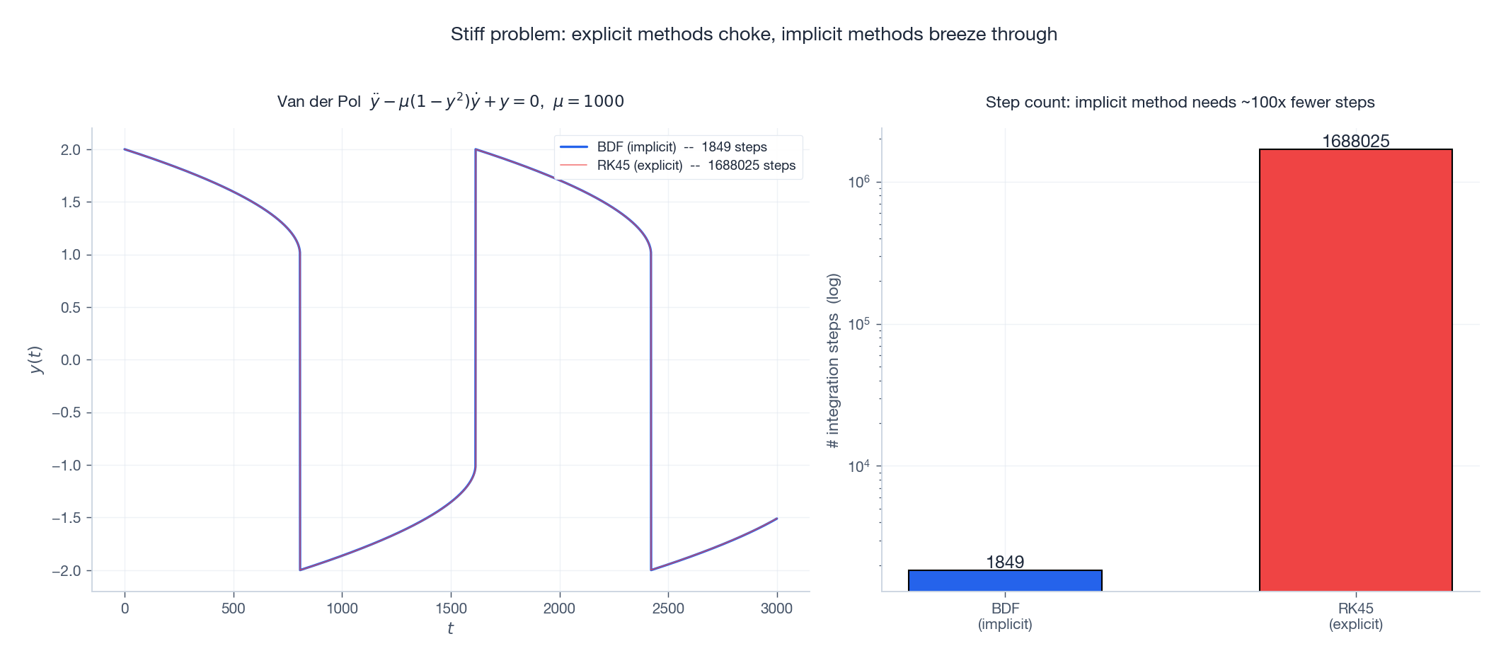
Stiffness: the failure mode of explicit methods#
Some equations have a small amount of fast dynamics living on top of a slow evolution. Once the fast part has decayed, you would like to take big steps — but explicit methods will not let you. They demand$h \lesssim 1/|\lambda_{\max}|$ forever, just to stay numerically stable. Such problems are called stiff.
The textbook example is the van der Pol oscillator at large nonlinearity:$\ddot{y} - \mu(1 - y^2)\dot{y} + y = 0.$ For$\mu = 1000$ , the slow timescale is$\sim \mu$ while the fast timescale is$\sim 1/\mu$ . The ratio is $10^6$ . Trying to integrate this with RK45 is a disaster.
The way out is implicit methods. The simplest is backward Euler:$y_{n+1} = y_n + h\,f(x_{n+1}, y_{n+1}),$ which evaluates the slope at the new point. The price: each step requires solving an algebraic equation for$y_{n+1}$ , usually by Newton’s method. The reward: backward Euler’s stability region is the entire left half-plane (it is A-stable). No matter how stiff the problem, you can take whatever$h$ is needed for accuracy.
Stability regions, drawn#
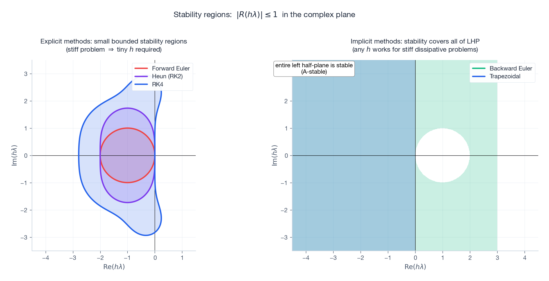
For a stiff problem with eigenvalues stretched far down the negative real axis, the explicit region is a narrow corridor. You either shrink$h$ enough to fit (huge cost) or use an A-stable method (no$h$ constraint).
In production, the standard implicit families are:
- BDF (Backward Differentiation Formulas, orders 1-5). The default for stiff ODEs in industrial solvers (LSODE, CVODE, SciPy’s
'BDF'). - Radau IIA (orders 3, 5, 9). Implicit Runge-Kutta with strong stability properties; SciPy’s
'Radau'. - Implicit midpoint / trapezoidal. A-stable, second order, energy-conserving for Hamiltonian systems.
A practical rule: if solve_ivp(..., method='RK45') is taking forever or refusing tolerances, try 'BDF' or 'Radau'. If the problem switches between stiff and non-stiff regimes, 'LSODA' does the detection automatically.
A few more methods worth knowing#
Multistep: Adams-Bashforth and Adams-Moulton#
Instead of evaluating$f$ at multiple internal stages, multistep methods reuse stored values from previous steps:$y_{n+1} = y_n + h \sum_{j=0}^{k-1} \beta_j\,f(x_{n-j}, y_{n-j}).$ Adams-Bashforth (explicit) and Adams-Moulton (implicit) are the textbook families. Predictor-corrector pairs combine an Adams-Bashforth prediction with an Adams-Moulton correction. The advantage is one function evaluation per step (after startup); the disadvantage is fragility around discontinuities and the need for separate startup procedures.
Symplectic integrators for Hamiltonian flows#
For energy-conserving systems (planetary orbits, molecular dynamics, lattice gauge theory), conventional methods cause energy drift: the conserved quantity slowly grows or shrinks as round-off accumulates. Symplectic integrators preserve the symplectic 2-form of phase space; they cannot conserve energy exactly either, but they confine the energy error to a bounded oscillation around the true value, even over millions of periods.
The minimal example is Störmer-Verlet (leapfrog) for$\ddot q = -\nabla V(q)$ :$p_{n+1/2} = p_n - \tfrac{h}{2}\nabla V(q_n),\quad q_{n+1} = q_n + h\,p_{n+1/2},\quad p_{n+1} = p_{n+1/2} - \tfrac{h}{2}\nabla V(q_{n+1}).$ Second-order accurate, time-reversible, symplectic. The standard tool of N-body astrophysics.
Using SciPy in practice#
| |
solve_ivp’s most-used options:
method:'RK45'(default),'RK23','DOP853'(8th-order, very high accuracy),'Radau','BDF','LSODA'.rtol,atol: relative and absolute tolerances per component. Defaults are loose ($10^{-3}, 10^{-6}$ ); for serious work tighten to$10^{-8}, 10^{-10}$ or below.dense_output=True: returns an interpolantsol.sol(t)you can call at any time, not just at the integrator’s chosen steps.events: pass a function and the solver locates its zeros via root-finding — ideal for collisions, bouncing, threshold crossings.jac: provide an analytic Jacobian for stiff methods; massive speedup over finite-difference Jacobians.
Practical reliability checklist#
- Run twice at different tolerances. If reducing
rtolby 100x changes the answer noticeably, the looser run was wrong. - Plot the step-size history. A solver hammering on
min_stepis in trouble. Ifnfev(function evaluations) is enormous, you are probably on a stiff problem with an explicit method. - Watch for
success=False.solve_ivpreturns this silently; you must check it. - For long integrations, use a dense output and verify on a coarser grid. Drift over$10^6$ periods is invisible in any single-step check.
Method selection summary#
| Method | Order | Class | Stable for stiff? | Best for |
|---|---|---|---|---|
| Forward Euler | 1 | explicit | no | learning, never production |
| Heun (improved Euler) | 2 | explicit | no | toy problems |
| Classical RK4 | 4 | explicit | no | smooth non-stiff problems |
| Dormand-Prince RK4(5) | 4(5) | explicit, adaptive | no | the default workhorse |
| DOP853 | 8(5,3) | explicit, adaptive | no | demanding non-stiff accuracy |
| Backward Euler | 1 | implicit | yes (A-stable) | minimal stiff solver |
| Trapezoidal / Crank-Nicolson | 2 | implicit | yes (A-stable) | mildly stiff, conservative |
| BDF (orders 1-5) | up to 5 | implicit, multistep | yes | stiff industrial workhorse |
| Radau IIA | 3, 5, 9 | implicit RK | yes (L-stable) | very stiff, high-accuracy |
| Störmer-Verlet | 2 | symplectic | — | Hamiltonian / orbital |
One sentence of advice: start with solve_ivp(method='RK45'); if it is slow or unstable, switch to 'BDF' and try again; if it conserves something and you care about that, look at symplectic methods.
Exercises#
- Order verification. Implement
euler,heun, andrk4. Solve$\dot y = -2y$ ,$y(0)=1$ on$[0, 3]$ at$h \in \{0.5, 0.25, 0.125, 0.0625\}$ , plot the global error log-log, and confirm slopes 1, 2, 4. - Stability boundary, by experiment. For Euler applied to$\dot y = \lambda y$ with$\lambda = -10$ , find the critical step size$h_*$ at which Euler stops being stable, and verify it agrees with$2/|\lambda|$ .
- A stiff system, both ways. Solve the Robertson chemical kinetics problem $ \dot y_1 = -0.04 y_1 + 10^4 y_2 y_3, $
with$y(0) = (1, 0, 0)$
on$[0, 10^{11}]$
using both 'RK45' and 'BDF'. Compare run time and step count.
4. Adaptive vs fixed. Use solve_ivp to integrate$\dot y = -y + 100\,e^{-(t-1)^2/0.005}$
on$[0, 3]$
at rtol=1e-6. Then redo with a fixed-step RK4 fine enough to match the accuracy. Report the step counts.
5. Symplectic vs RK4 on the Kepler orbit. Integrate a circular Kepler orbit for$10^4$
periods using leapfrog and using RK4 at the same step size. Plot energy vs time for each.
References#
- Hairer, E., Norsett, S. P., & Wanner, G. (1993). Solving Ordinary Differential Equations I: Nonstiff Problems (2nd ed.). Springer.
- Hairer, E. & Wanner, G. (1996). Solving Ordinary Differential Equations II: Stiff and Differential-Algebraic Problems (2nd ed.). Springer. The two Hairer-Wanner volumes are the bible.
- Ascher, U. & Petzold, L. (1998). Computer Methods for Ordinary Differential Equations and Differential-Algebraic Equations. SIAM.
- Hairer, E., Lubich, C. & Wanner, G. (2006). Geometric Numerical Integration (2nd ed.). Springer. The reference for symplectic methods.
- SciPy documentation:
scipy.integrate.solve_ivpand the source of its method classes.
Previous Chapter: Chapter 10: Bifurcation Theory
Next Chapter: Chapter 12: Boundary Value Problems
This is Part 11 of the 18-part series on Ordinary Differential Equations.
ODE Foundations 18 parts
- 01 Ordinary Differential Equations (1): Origins and Intuition
- 02 Ordinary Differential Equations (2): First-Order Methods
- 03 Ordinary Differential Equations (3): Higher-Order Linear Theory
- 04 Ordinary Differential Equations (4): The Laplace Transform
- 05 Ordinary Differential Equations (5): Power Series and Special Functions
- 06 Ordinary Differential Equations (6): Linear Systems and the Matrix Exponential
- 07 Ordinary Differential Equations (7): Stability Theory
- 08 Ordinary Differential Equations (8): Nonlinear Systems and Phase Portraits
- 09 Ordinary Differential Equations (9): Chaos Theory and the Lorenz System
- 10 Ordinary Differential Equations (10): Bifurcation Theory
- 11 Ordinary Differential Equations (11): Numerical Methods you are here
- 12 Ordinary Differential Equations (12): Boundary Value Problems
- 13 Ordinary Differential Equations (13): Introduction to Partial Differential Equations
- 14 Ordinary Differential Equations (14): Epidemic Models and Epidemiology
- 15 Ordinary Differential Equations (15): Population Dynamics
- 16 Ordinary Differential Equations (16): Fundamentals of Control Theory
- 17 Ordinary Differential Equations (17): Physics and Engineering Applications
- 18 Ordinary Differential Equations (18): Frontiers and Series Finale