Ordinary Differential Equations (12): Boundary Value Problems

An initial value problem hands you a starting state and asks you to march forward. A boundary value problem (BVP) hands you partial information at two different points and asks you to find a path that fits both. The change is small in wording, large in consequence: BVPs can have a unique solution, no solution at all, or infinitely many. They demand a fundamentally different toolkit – one that is iterative, global, and intimately connected to linear algebra.

This is also where ODE methods quietly become PDE methods. The discretization, eigenvalue, and collocation ideas you meet here scale directly to elliptic PDEs in higher dimensions.

What you will learn

Why BVPs are qualitatively harder than IVPs, with a worked example showing existence and uniqueness can both fail
Three standard boundary-condition types: Dirichlet, Neumann, Robin
The shooting method – reducing a BVP to a root-finding problem on the missing initial condition
The finite-difference method – reducing a BVP to a sparse linear system
Sturm-Liouville theory and how it makes BVPs into matrix eigenvalue problems (the bridge to quantum mechanics and vibration analysis)
A taste of collocation via scipy.integrate.solve_bvp, the standard Python tool

Prerequisites: numerical methods from Chapter 11 .

1. From IVP to BVP: a small change with big consequences

The canonical second-order BVP is$y'' = f(x, y, y'), \quad y(a) = \alpha, \quad y(b) = \beta.$Compare with the IVP, which would specify$y(a) = \alpha,\;y'(a) = \alpha'$. The data set is the same size (two scalars), but its distribution matters enormously.

For an IVP under mild Lipschitz conditions, Picard’s theorem guarantees existence and uniqueness. The flow exists, period. For a BVP, none of that is guaranteed.

The pedagogical example everybody uses

Take$y'' + y = 0$with various boundary conditions:

boundary conditions	solutions
$y(0)=0,\;y(\pi)=0$	infinitely many:$y = A\sin x$for any$A$
$y(0)=0,\;y(\pi)=1$	none (every$\sin x$is zero at$x=\pi$)
$y(0)=0,\;y(1)=1$	unique:$y = \sin(x) / \sin(1)$

Same equation, three radically different fates. The reason is that$\sin x$happens to vanish at$x=\pi$– which means the homogeneous problem has a non-trivial solution, which by the Fredholm alternative is exactly when the inhomogeneous problem is either over- or under-determined. For BVPs, existence and uniqueness depend on the boundary data, not just the equation.

Three flavors of boundary conditions

Dirichlet (function values):$y(a) = \alpha,\;y(b) = \beta$. Temperature held at the endpoints. The default.
Neumann (derivative values):$y'(a) = \alpha,\;y'(b) = \beta$. Heat flux specified, or a free end of a beam.
Robin (linear combination):$\alpha_1 y(a) + \alpha_2 y'(a) = \gamma$. Newton’s law of cooling, partial absorption.

Mixed types are common in practice (Dirichlet on one side, Neumann on the other). The numerical methods we develop handle all three with minor modifications.

2. The shooting method

The simplest idea in the book: turn the BVP into a parametric IVP. For a second-order BVP we know$y(a) = \alpha$but not$y'(a)$. Pick a guess$s$, integrate the IVP$y'' = f(x, y, y'), \quad y(a) = \alpha, \quad y'(a) = s$forward to$x = b$, and look at the residual$F(s) := y(b; s) - \beta$. We want$F(s) = 0$. That is a one-dimensional root-finding problem, solvable by bisection, secant, Newton, or brentq.

Shooting method: trial trajectories and the residual function whose root is the right initial slope.

Left: the BVP$y''+y=0,\;y(0)=0,\;y(\pi/2)=1$. Five trial slopes give five trajectories; only$s=1$lands on the target marker. Right: the residual$F(s) = y(\pi/2; s) - 1$. Shooting reduces the BVP to finding the zero of this curve.

The geometric picture is exactly that of an artillery officer ranging a gun: you fire shells with different initial elevations and adjust until one lands on the target. The same metaphor gives the method its name.

 1
 2
 3
 4
 5
 6
 7
 8
 9
10
11
12
13
14
15
16
17
18
19
20
21
22
import numpy as np
from scipy.integrate import solve_ivp
from scipy.optimize import brentq

def shooting_method(f, a, b, alpha, beta, s_low=-10, s_high=10):
    """Solve y'' = f(x, y, y'), y(a)=alpha, y(b)=beta, by shooting."""
    def residual(s):
        sol = solve_ivp(lambda x, Y: [Y[1], f(x, Y[0], Y[1])],
                        [a, b], [alpha, s], dense_output=True,
                        rtol=1e-9, atol=1e-12)
        return sol.sol(b)[0] - beta

    # Bracket-expand if needed
    while residual(s_low) * residual(s_high) > 0:
        s_low, s_high = s_low * 2, s_high * 2

    s_opt = brentq(residual, s_low, s_high, xtol=1e-10)
    sol = solve_ivp(lambda x, Y: [Y[1], f(x, Y[0], Y[1])],
                    [a, b], [alpha, s_opt], dense_output=True,
                    rtol=1e-9, atol=1e-12)
    x_out = np.linspace(a, b, 200)
    return x_out, sol.sol(x_out)[0]

When shooting works – and when it does not

Shooting is excellent when the underlying IVP is well-conditioned: small changes in$s$produce small changes in$y(b)$, so root-finding has a clean target. It is terrible when the IVP amplifies errors exponentially – a common scenario near singular perturbations or for stiff problems with growing modes. Try shooting$y'' - 100y = 0$on$[0, 10]$with$y(0) = 0, y(10) = 1$: the$\sinh$mode contaminates everything, and the residual$F(s)$ranges over $\sim 10^{43}$, making accurate root-finding impossible.

The standard cure is multiple shooting: divide$[a, b]$into$M$panels, shoot independently on each (with both endpoints as unknowns), and add matching equations between panels. The resulting nonlinear system is larger but each individual shot is short and well-conditioned.

3. The finite-difference method

A different philosophy: discretize the operator first, then solve. On a uniform grid$x_i = a + ih,\;i=0,\ldots,N,\;h = (b-a)/N$, central differences give$y'(x_i) \approx \frac{y_{i+1} - y_{i-1}}{2h}, \qquad y''(x_i) \approx \frac{y_{i+1} - 2y_i + y_{i-1}}{h^2}.$Substituting into the BVP at every interior node$i = 1,\ldots,N-1$turns it into a system of$N-1$equations in$N-1$unknowns$y_1, \ldots, y_{N-1}$(with$y_0 = \alpha$and$y_N = \beta$absorbed into the right-hand side).

For a linear BVP$y'' + p(x) y' + q(x) y = r(x)$the system is tridiagonal, with one super- and one sub-diagonal. Solving an$n\times n$tridiagonal system costs$\mathcal{O}(n)$rather than the$\mathcal{O}(n^3)$of generic Gaussian elimination.

Finite-difference solution and the tridiagonal sparsity pattern.

Left: numerical solution of$y'' = -\pi^2 \sin(\pi x)$on$[0, 1]$with$y(0) = y(1) = 0$, exact answer$\sin(\pi x)$. Three highlighted dots show the local 3-point stencil. Right: structure of$h^2 A$. Only three non-zero diagonals; everything else is exactly zero. Memory and CPU cost are both$\mathcal{O}(N)$.

For nonlinear BVPs the discretization yields a nonlinear algebraic system, solved by Newton iteration. The Newton Jacobian inherits the same sparsity, so each Newton step still costs$\mathcal{O}(N)$.

 1
 2
 3
 4
 5
 6
 7
 8
 9
10
11
12
13
14
15
16
17
18
19
20
21
22
23
24
25
26
27
28
29
30
31
32
import numpy as np
from scipy.linalg import solve_banded

def finite_difference_linear(p, q, r, a, b, alpha, beta, N):
    """
    Solve y'' + p(x)y' + q(x)y = r(x), y(a)=alpha, y(b)=beta
    by central differences on a uniform grid of N intervals.

    Returns the grid x and the discrete solution y.
    """
    h = (b - a) / N
    x = np.linspace(a, b, N + 1)
    n = N - 1
    pi = np.array([p(xi) for xi in x[1:-1]])
    qi = np.array([q(xi) for xi in x[1:-1]])
    ri = np.array([r(xi) for xi in x[1:-1]])

    main = -2 / h**2 + qi
    upper = 1 / h**2 + pi[:-1] / (2 * h)
    lower = 1 / h**2 - pi[1:]  / (2 * h)

    rhs = ri.copy()
    rhs[0]  -= (1 / h**2 - pi[0]  / (2 * h)) * alpha
    rhs[-1] -= (1 / h**2 + pi[-1] / (2 * h)) * beta

    ab = np.zeros((3, n))
    ab[0, 1:] = upper
    ab[1, :]  = main
    ab[2, :-1] = lower

    y_int = solve_banded((1, 1), ab, rhs)
    return x, np.concatenate([[alpha], y_int, [beta]])

Convergence

Central differences are second-order: the truncation error is$\mathcal{O}(h^2)$, so halving$h$cuts the error to a quarter. To get fourth-order accuracy you can use compact (Pade) finite differences or Numerov’s method (a tailored scheme for$y'' = f(x, y)$); to get spectral accuracy you can use Chebyshev collocation – but at the cost of dense matrices.

4. Eigenvalue problems

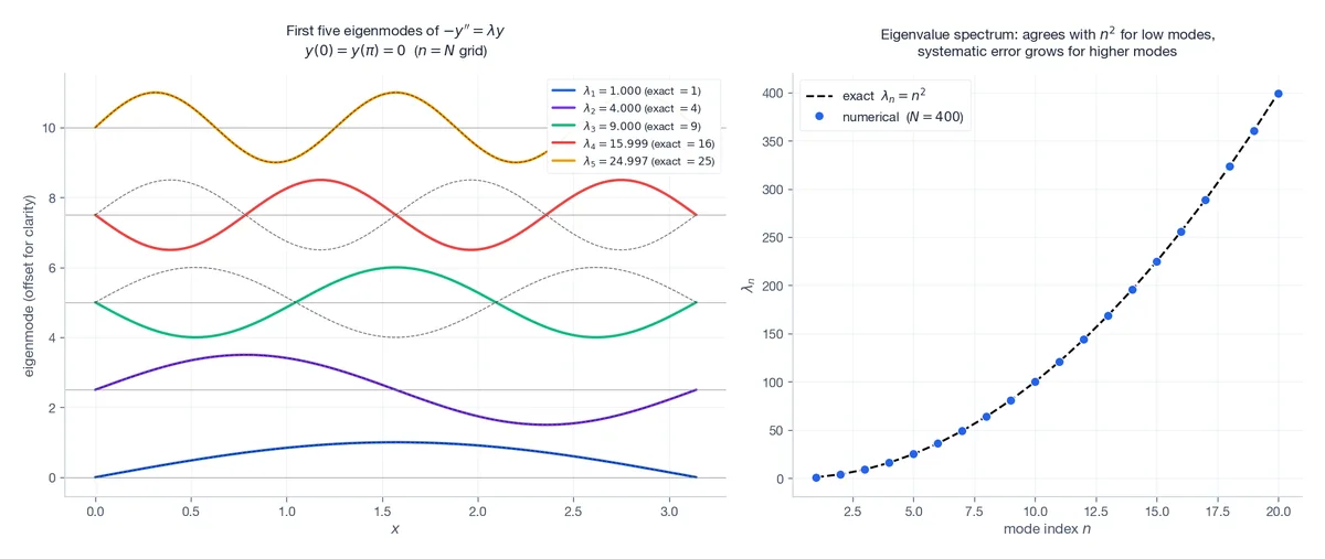
Linear BVPs with homogeneous boundary conditions and a parameter$\lambda$in the equation are eigenvalue problems. The simplest case:$-y'' = \lambda y, \quad y(0) = y(\pi) = 0.$Direct calculation gives eigenvalues$\lambda_n = n^2$with eigenfunctions$\sin(nx)$,$n = 1, 2, 3, \ldots$.

After finite-difference discretization, the operator$-y''$becomes a symmetric tridiagonal matrix. Its eigenvalues approximate$\{\lambda_n\}$, accurately for low modes (long wavelengths) and progressively worse for high modes (the grid cannot resolve oscillations finer than$2h$).

First five eigenmodes and the spectrum compared with the exact n-squared rule.

Left: the first five computed eigenmodes (colored solid) and the exact$\sin(nx)$(black dashed), offset for clarity. Numerical eigenvalues to four decimal places match$1, 4, 9, 16, 25$. Right: low modes lie exactly on the curve$\lambda_n = n^2$; the systematic dispersion error grows as$n$approaches the grid limit.

 1
 2
 3
 4
 5
 6
 7
 8
 9
10
11
12
from scipy.linalg import eigh_tridiagonal
import numpy as np

# -y'' = lambda y, y(0) = y(pi) = 0, on N intervals
N = 400
h = np.pi / N
n = N - 1
main = (2 / h**2) * np.ones(n)
off  = (-1 / h**2) * np.ones(n - 1)
eigvals, eigvecs = eigh_tridiagonal(main, off, select='i',
                                    select_range=(0, 9))
print(eigvals.round(4))    # [1.0000  4.0000  9.0000 16.0000 25.0000 ...]

5. Sturm-Liouville theory

The general second-order self-adjoint eigenvalue problem is$-\bigl(p(x)\,y'\bigr)' + q(x)\,y = \lambda\,w(x)\,y, \quad y(a) = y(b) = 0,$with$p>0$,$w>0$. This is the Sturm-Liouville form, and it is the bridge from ODEs to mathematical physics.

Properties (for regular Sturm-Liouville problems on a finite interval):

Real, simple, ordered eigenvalues$\lambda_1 < \lambda_2 < \lambda_3 < \cdots \to \infty$.
Orthogonality:$\int_a^b w(x) y_m(x) y_n(x)\,dx = 0$for$m \ne n$.
Completeness: any sufficiently smooth function satisfying the boundary conditions can be expanded as$f(x) = \sum_n c_n y_n(x)$with$c_n = \int w f y_n / \int w y_n^2$.
Oscillation theorem: the$n$-th eigenfunction$y_n$has exactly$n-1$zeros in the open interval$(a, b)$.

These are the same properties that make Fourier series, Bessel-function expansions, Legendre series, and quantum-mechanical bound states all work. They are the right way to think about every “expansion in eigenfunctions” you will ever do.

A worked example: the quantum harmonic oscillator

Schrodinger’s equation in dimensionless form for the harmonic oscillator:$-\psi''(x) + x^2\,\psi(x) = E\,\psi(x), \quad \psi(\pm\infty) = 0.$This is Sturm-Liouville with$p \equiv 1$,$q(x) = x^2$,$w \equiv 1$on the unbounded domain. Exact eigenvalues:$E_n = 2n + 1$for$n = 0, 1, 2, \ldots$. Eigenfunctions are Hermite functions.

We solve numerically by truncating the domain to$[-L, L]$with$L$large enough that$\psi$is essentially zero at the boundary, discretizing with central differences, and asking for the lowest few eigenvalues of the resulting matrix.

First five eigenfunctions of the quantum harmonic oscillator overlaid on the parabolic potential.

The black curve is the potential$V(x) = x^2$. Each colored eigenfunction is plotted at the height of its energy$E_n$, showing the classic structure: each next mode adds one node, and the wavefunctions oscillate inside the classical turning points and decay exponentially outside. Numerical eigenvalues match the exact$2n+1$to four decimals.

This template – “discretize, eigh, plot at energy” – is essentially the entire toolkit for one-dimensional bound-state problems in quantum mechanics. The same machinery yields the modes of vibrating strings, drums, and molecules.

6. Collocation: scipy.integrate.solve_bvp

Modern production BVP solvers usually use collocation rather than shooting or finite differences. The idea: assume the solution is a piecewise polynomial on a mesh, and demand that it satisfy the ODE exactly at chosen “collocation” points within each interval. SciPy’s solve_bvp implements a 4th-order Lobatto IIIa scheme with adaptive mesh refinement.

The user provides:

fun(x, y): the right-hand side as a first-order system, vectorized.
bc(ya, yb): residual of the boundary conditions, returning an array of length equal to the system size.
x and y_init: an initial mesh and a guess.

 1
 2
 3
 4
 5
 6
 7
 8
 9
10
11
12
13
14
15
16
from scipy.integrate import solve_bvp
import numpy as np

# Bratu problem:  y'' + lambda * exp(y) = 0,  y(0) = y(1) = 0,  lambda = 2
def fun(x, y):
    return np.vstack([y[1], -2 * np.exp(y[0])])

def bc(ya, yb):
    return np.array([ya[0], yb[0]])      # both endpoints zero

x_init = np.linspace(0, 1, 10)
y_init = np.zeros((2, x_init.size))
y_init[0] = 0.5 * np.sin(np.pi * x_init)        # bump-shaped guess

sol = solve_bvp(fun, bc, x_init, y_init, tol=1e-10)
assert sol.success

solve_bvp’s strengths:

adaptive mesh refinement – it places nodes where the solution varies fastest;
handles nonlinear BVPs natively via Newton iteration on the collocation residual;
the result sol.sol is a continuous, differentiable spline you can evaluate anywhere.

Its weaknesses: like all global methods, it requires a reasonable initial guess; a pathological guess can drive Newton to a different solution branch (or to no solution at all).

7. Putting it all together: same problem, three methods

The famous Bratu problem$y'' + 2 e^{y} = 0$,$y(0) = y(1) = 0$has two solutions on the lower branch (a small one and a larger one); we focus on the small one.

Three independent BVP methods on the Bratu problem; all agree to plotting accuracy.

Left: shooting + brentq, finite differences + Newton, and solve_bvp collocation – three different algorithms, three different numerical pipelines, one solution. Right: the pairwise differences are at the$10^{-7}$level, dominated by each method’s own tolerance settings.

The redundancy is reassuring. When two independent BVP methods disagree by something other than tolerance, one of them is wrong; usually it is shooting hitting a sensitivity wall, or solve_bvp being trapped in the wrong branch by a bad guess.

8. Where this leads: applications

Beam deflection. Euler-Bernoulli beam:$EI\,y^{(4)} = w(x)$with combinations of fixed/free/simply-supported boundary conditions. Eigenvalues give the natural vibration frequencies of the beam; eigenfunctions are mode shapes used in structural dynamics.
Steady heat conduction.$(k(x) T'(x))' + Q(x) = 0$with Dirichlet (prescribed temperature) or Neumann (prescribed flux) boundaries. Sturm-Liouville to the bone; eigenfunction expansions give the time-dependent heat equation by separation of variables.
Quantum bound states. As above. Add a finite well, a periodic potential, a hydrogenic Coulomb tail – the numerical recipe is identical, just change$V(x)$.
Thomas-Fermi, Bratu, Falkner-Skan, blasius, Painleve. Classical nonlinear BVPs with rich histories. All of them yield to solve_bvp if you start with a reasonable guess.
Two-point optimal control. Pontryagin’s maximum principle turns optimal control problems into BVPs in the state-costate system. Multiple shooting is the workhorse here.

The same finite-difference and collocation ideas extend to elliptic PDEs (Laplace, Poisson, Helmholtz) in two and three dimensions. The matrices stop being tridiagonal but stay sparse; iterative solvers (multigrid, Krylov) handle the linear algebra. Everything you have learned about BVPs scales up.

9. Method selection summary

Method	Best for	Watch out for
Shooting	Well-conditioned IVPs, simple problems	Sensitivity / stiffness blowup
Multiple shooting	Sensitive problems, two-point optimal control	More setup, larger nonlinear system
Finite difference	Linear problems, eigenvalue problems	Order limited to 2 (or higher with extra work)
Spectral / Chebyshev	Smooth solutions, high accuracy	Requires careful basis choice
Collocation (`solve_bvp`)	General nonlinear BVPs	Needs reasonable initial guess

Practical default: use solve_bvp for new BVPs. If it fails, the problem is usually the initial guess, not the method.

Exercises

Existence/uniqueness experiment. Numerically attempt the BVP$y'' + y = 0$with$y(0) = 0$,$y(\pi) = 1$using solve_bvp. Document what happens and explain it via the Fredholm alternative.
Convergence of finite differences. Solve$y'' = -\pi^2 \sin(\pi x)$,$y(0) = y(1) = 0$at$N \in \{20, 40, 80, 160, 320\}$. Plot the maximum error vs$h$on log-log axes and confirm slope 2.
Quantum well. Compute the lowest five eigenvalues and eigenfunctions of$-\psi'' + V(x)\psi = E\psi$on$[-10, 10]$with$V(x) = -10\,e^{-x^2/2}$. How many bound states ($E < 0$) does this Gaussian well support?
Multiple shooting. Solve$y'' = 100\,y$,$y(0) = 0$,$y(1) = 1$by single shooting (it should fail or be very inaccurate). Then split$[0, 1]$into 5 panels and use multiple shooting; verify that the result matches$y = \sinh(10x)/\sinh(10)$.
A nonlinear example. Use solve_bvp to find both branches of the Bratu problem$y'' + \lambda e^y = 0$,$y(0) = y(1) = 0$at$\lambda = 2$. (Hint: try two different initial guesses for the bump amplitude.)

References

Ascher, U. M., Mattheij, R. M. M., & Russell, R. D. (1995). Numerical Solution of Boundary Value Problems for Ordinary Differential Equations. SIAM Classics.
Keller, H. B. (1976). Numerical Solution of Two Point Boundary Value Problems. SIAM.
Boyd, J. P. (2001). Chebyshev and Fourier Spectral Methods (2nd ed.). Dover.
LeVeque, R. J. (2007). Finite Difference Methods for Ordinary and Partial Differential Equations. SIAM.
SciPy documentation: scipy.integrate.solve_bvp.

Previous Chapter: Chapter 11: Numerical Methods

Next Chapter: Chapter 13: Introduction to Partial Differential Equations

This is Part 12 of the 18-part series on Ordinary Differential Equations.