Ordinary Differential Equations (13): Introduction to Partial Differential Equations
Step from ODEs into partial differential equations. Classify PDEs into parabolic, hyperbolic, and elliptic types. Solve the heat, wave, and Laplace equations using separation of variables and finite differences.
Once a quantity depends on more than one variable, the ODE world splinters into a vastly richer one: partial differential equations. Heat in a metal rod is a function of position and time; a vibrating string moves in space and time; a steady electrostatic potential lives in three spatial dimensions. ODE techniques become tools, not solutions — separation of variables turns one PDE into a family of ODEs, the eigenvalues of those ODEs become the spectrum of the operator, and superposition stitches everything back together.
This chapter is a working tour, not an encyclopaedia: we focus on the three classical equations — heat, wave, Laplace — because every linear second-order PDE in two variables is similar, in a precise sense, to one of them.

What You Will Learn#
- How PDEs differ qualitatively from ODEs and why three “canonical types” cover almost everything linear
- The classification theorem: discriminant $B^2 - AC$ as the parabolic / hyperbolic / elliptic detector
- Separation of variables as a recipe: PDE -> Sturm-Liouville eigenproblem -> Fourier series
- d’Alembert’s formula and the light cone — finite vs infinite propagation speed
- Finite differences (FTCS, Crank-Nicolson, leapfrog) and what makes them stable (CFL, von Neumann)
- The maximum principle and Gauss-Seidel iteration for the Laplace equation
- A first taste of well-posedness: which initial / boundary data make a PDE problem solvable
Prerequisites: ODE methods through Chapter 11 , Chapter 12 boundary value problems , and basic multivariable calculus (gradient, Laplacian, chain rule).
From ODEs to PDEs#
In an ODE, the unknown $y(t)$ depends on a single variable. Every solution is parametrised by finitely many constants — one per order of differentiation — and an initial condition picks one out.
A PDE asks for a function of several variables. Specifying it requires data along an entire lower-dimensional surface (a curve in 2D, a surface in 3D), and the resulting solution space is genuinely infinite-dimensional. The same equation can be well-posed with one kind of data and ill-posed with another — a phenomenon that has no ODE analogue.
The classical trio#
| Equation | Formula | Type | Physics |
|---|---|---|---|
| Heat | $u_t = \alpha\,u_{xx}$ | parabolic | irreversible diffusion |
| Wave | $u_{tt} = c^2\,u_{xx}$ | hyperbolic | reversible propagation |
| Laplace | $u_{xx} + u_{yy} = 0$ | elliptic | equilibrium / no time |
Why exactly these three? Because every linear second-order PDE in two variables can, by a change of coordinates, be brought into one of three canonical forms. The discriminant decides which.
Classification#
$$ A\,u_{xx} + 2B\,u_{xy} + C\,u_{yy} + (\text{lower order}) = 0, $$form the discriminant $\Delta = B^2 - AC$ . Then:
| $\Delta$ | Type | Canonical example | Real characteristics? |
|---|---|---|---|
| $> 0$ | hyperbolic | wave equation | two families |
| $= 0$ | parabolic | heat equation | one family (degenerate) |
| $< 0$ | elliptic | Laplace equation | none (complex) |
The number of real characteristic curves controls how disturbances propagate, what data the problem accepts, and which numerical schemes work.

Top-left: the $(AC, B^2)$ plane sliced by the line $B^2 = AC$ — above is hyperbolic, below is elliptic, on it is parabolic. Top-middle: the parabolic fundamental solution — a $\delta$ -source at the origin smears out as a Gaussian, instantly nonzero everywhere (formal “infinite speed”). Top-right: the hyperbolic case — a localised disturbance is contained in a finite-speed light cone $|x| \leq ct$ . Bottom row: the three canonical equations side by side, with their distinguishing properties.
Physical intuition.
- Hyperbolic. Drop a stone in a pond — ripples move at finite speed; signals reach a point only after a delay.
- Parabolic. Touch one end of a steel rod — in theory the other end heats up instantly (although exponentially weakly).
- Elliptic. Steady state. Time has been integrated out; only equilibrium between sources and sinks remains.
Even though the parabolic “infinite speed” is unphysical for real materials, the model is excellent in practice because the front decays so fast that no measurable effect arrives until it should.
The Heat Equation#
Derivation in one paragraph#
$$ \rho c_p \frac{\partial u}{\partial t} = -\frac{\partial q}{\partial x}, $$ $$ u_t = \alpha\,u_{xx}, \qquad \alpha = \frac{k}{\rho c_p}. $$The diffusivity $\alpha$ has units $\text{length}^2 / \text{time}$ — the only natural way to combine $k$ , $\rho$ , $c_p$ .
Separation of variables#
$$ \frac{T'}{\alpha T} = \frac{X''}{X} = -\lambda \quad (\text{constant}). $$ $$X'' + \lambda X = 0, \qquad T' + \alpha\lambda\,T = 0.$$ $$\boxed{\;u(x, t) = \sum_{n=1}^\infty b_n\,\sin\!\frac{n\pi x}{L}\,e^{-\alpha (n\pi / L)^2 t},\quad b_n = \frac{2}{L}\int_0^L f(x)\sin\!\frac{n\pi x}{L}\,dx.\;}$$Two structural lessons:
- The heat equation is a Fourier filter. High modes (large $n$ ) decay much faster than low modes — mode $n$ has half-life $\propto 1/n^2$ . Sharp features in the initial condition are erased almost immediately; smooth features linger.
- Boundary conditions select a basis. Dirichlet -> sines, Neumann -> cosines, periodic -> complex exponentials. The eigenfunctions are orthogonal, so coefficients are inner products. This is the spectral decomposition of the Laplacian.

Left: snapshots of $u(x, t)$ at six times — a piecewise-constant initial profile is smoothed within fractions of a second and approaches the equilibrium $u \equiv 0$ . Middle: the same solution as a spacetime heatmap — bright structures fade upward in time. Right: log-scale decay of the Fourier modes; mode $n = 10$ is a thousand times faster than $n = 1$ . The heat equation is a low-pass filter.
Separation of variables, visualised#
Each ingredient of the recipe deserves its own picture. The eigenfunctions are spatial standing patterns; the time factors are decay envelopes; their products are the elementary solutions; superposition recovers the initial data.
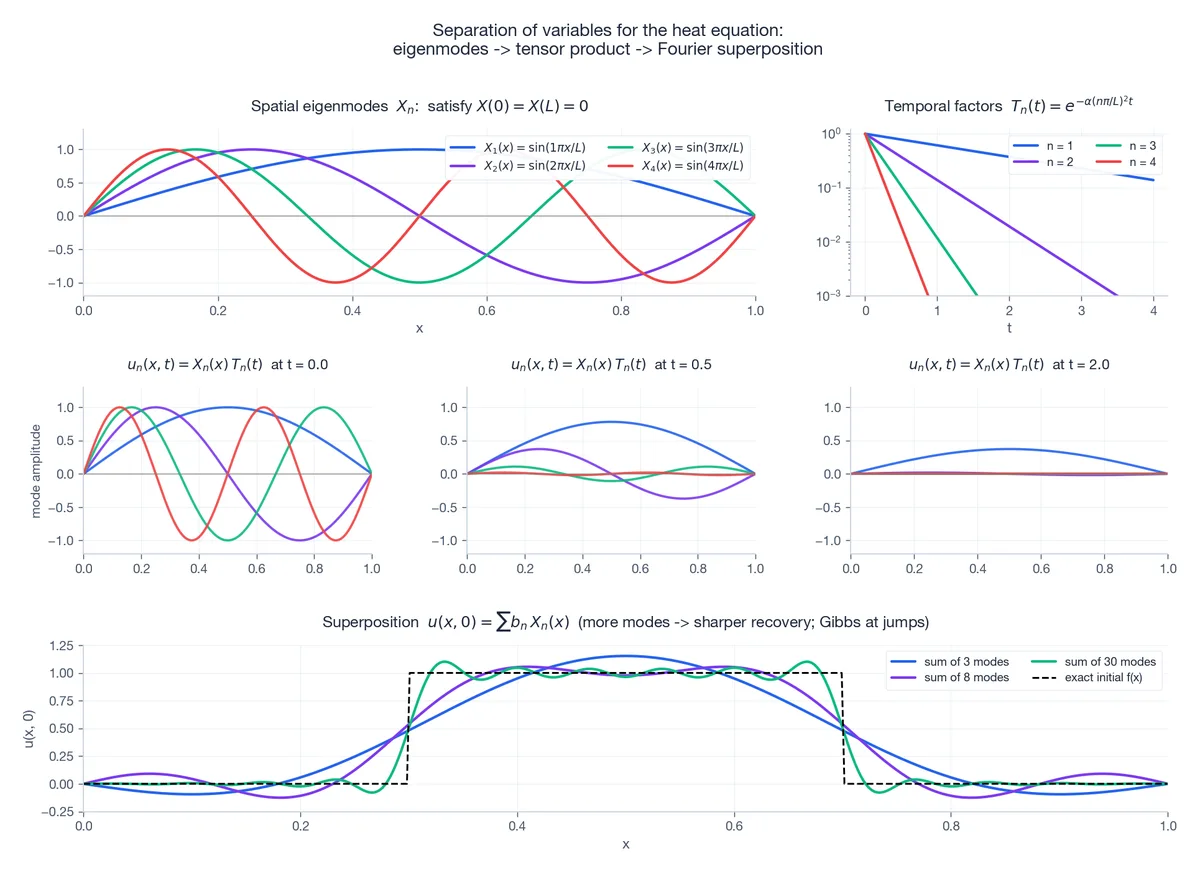
Top-left: spatial eigenmodes $X_n(x) = \sin(n\pi x/L)$ — they vanish at the endpoints by construction. Top-right: the matching temporal factors $T_n(t)$ , decaying faster for larger $n$ . Middle row: the elementary solutions $u_n(x, t) = X_n T_n$ at three times — short-wavelength modes have nearly disappeared by $t = 2$ . Bottom: reconstructing a square-pulse initial condition from progressively more modes. With three modes the shape is barely sketched; with thirty modes the agreement is excellent everywhere except near the jumps, where the Gibbs phenomenon persists.
Finite differences for the heat equation#
Discretise $x_j = j\,\Delta x$ and $t^n = n\,\Delta t$ . Three workhorse schemes, each a one-line update plus a stability story:
$$ u_j^{n+1} = u_j^n + r\,(u_{j+1}^n - 2u_j^n + u_{j-1}^n), \qquad r = \frac{\alpha\,\Delta t}{\Delta x^2}. $$Von Neumann analysis (substitute $u_j^n = \xi^n e^{ik j \Delta x}$ and demand $|\xi| \leq 1$ ) gives the stability constraint $r \leq 1/2$ . Halving $\Delta x$ forces $\Delta t$ to be quartered — accuracy is cheap, stability is expensive.
BTCS (Backward Time, Centred Space). Implicit, $O(\Delta t, \Delta x^2)$ , unconditionally stable: $|\xi| \leq 1$ for any $r > 0$ . Each step solves a tridiagonal system.
Crank-Nicolson. Average FTCS and BTCS; $O(\Delta t^2, \Delta x^2)$ , unconditionally stable, and the gold standard for the linear heat equation.
| |
The Wave Equation#

d’Alembert and the light cone#
$$ \boxed{\;u(x, t) = \frac{1}{2}\bigl[f(x - ct) + f(x + ct)\bigr] + \frac{1}{2c}\int_{x - ct}^{x + ct} g(s)\,ds.\;} $$Two observations rewrite the meaning of “wave”:
- The solution at $(x, t)$ depends only on data inside the interval of dependence $[x - ct, x + ct]$ . Anything outside that interval is invisible — finite signal speed.
- The two terms $f(x \pm ct)$ are travelling waves: rigid translations to the right and left. A bump released from rest splits into two half-amplitude bumps that move apart at speed $c$ .
Standing waves on a finite string#
$$ u(x, t) = \sum_{n=1}^\infty \bigl[a_n \cos(n\pi c\,t/L) + b_n \sin(n\pi c\,t/L)\bigr]\sin(n\pi x/L). $$The $n$ th mode oscillates at frequency $\omega_n = n\pi c / L$ . Mode 1 is the fundamental; modes $n \geq 2$ are harmonics. This is why a clarinet sounds different from a violin even at the same pitch — the amplitudes of the harmonics differ.
Numerical scheme and the CFL condition#
$$ u_j^{n+1} = 2u_j^n - u_j^{n-1} + \sigma^2(u_{j+1}^n - 2u_j^n + u_{j-1}^n), \qquad \sigma = \frac{c\,\Delta t}{\Delta x}. $$Von Neumann analysis gives the famous CFL condition $\sigma \leq 1$ . The geometric reading is gorgeous: the numerical domain of dependence at $(x, t)$ — the lattice points the scheme can possibly use — must contain the physical domain of dependence $[x - ct, x + ct]$ . If $\sigma > 1$ , the physical signal arrives faster than the numerical mesh can carry it, and the scheme blows up.

Top row: (a) a Gaussian pulse splitting into two half-amplitude pulses moving in opposite directions; (b) standing wave for $n = 3$ on a fixed-end string — three loops, two interior nodes; (c) a spacetime heatmap with the dashed light cone $x = \pm ct$ — everything outside the cone is identically zero. Bottom row: (d) leapfrog snapshots with $\sigma = 0.7$ — clean propagation; (e) the same scheme with $\sigma = 1.05$ — numerical chaos within half a unit of time; (f) the characteristic web $x \pm ct = \text{const}$ , along which information flows.
The Laplace Equation#
Time-independent equilibrium#
$\nabla^2 u = u_{xx} + u_{yy} = 0$ describes a steady distribution — temperature in a slab whose boundary is held fixed for so long that transients have died out, the gravitational potential outside masses, the velocity potential of an irrotational fluid. There is no time evolution; the only data are boundary conditions.
Two structural results#
$$ \min_{\partial\Omega} u \leq u(\mathbf{x}) \leq \max_{\partial\Omega} u \quad \text{for all } \mathbf{x} \in \Omega. $$The interior cannot be hotter than the hottest point on the boundary (and not colder than the coldest). The proof, in two lines, is a corollary of the mean-value property: $u(\mathbf{x}_0)$ equals the average of $u$ over any disc centred at $\mathbf{x}_0$ that fits in $\Omega$ . An interior maximum would have to equal its neighbours — so the maximum is constant in a neighbourhood, and a connectedness argument propagates it to the boundary.
Uniqueness. Two solutions with the same boundary data have a difference whose boundary values vanish — and by the maximum principle the difference is identically zero. So a Laplace BVP has exactly one solution.
Numerics: the five-point stencil#
$$ u_{i, j} = \frac{1}{4}\bigl(u_{i+1, j} + u_{i-1, j} + u_{i, j+1} + u_{i, j-1}\bigr). $$The discrete maximum principle is just an averaging statement — and it gives the recipe: starting from any guess, repeatedly replace each interior value by the average of its neighbours (Jacobi / Gauss-Seidel). For square grids of size $N$ this needs $O(N^2)$ iterations; SOR with optimal relaxation parameter brings it down to $O(N \log N)$ . For real work one uses multigrid or sparse direct solvers, but the iterative method is what the maximum principle suggests.

Left: solution to $\nabla^2 u = 0$ with a hot Gaussian bump on the top edge and zero on the other three. Heat penetrates downward and spreads laterally. Middle: equipotentials $u = \text{const}$ together with the negative gradient $-\nabla u$ , which (by Fourier’s law) is the heat-flux direction. Right: 600 random interior samples plotted against their $x$ -coordinate. Every single value lies below the boundary maximum and above the boundary minimum — the maximum principle in action.
Poisson equation#
Add a source: $\nabla^2 u = -f$ . The five-point stencil becomes $u_{i,j} = \tfrac{1}{4}(\text{neighbours}) + \tfrac{\Delta x^2}{4} f_{i,j}$ . Green’s functions reduce the continuous problem to convolution with the fundamental solution $G(\mathbf{x}, \mathbf{y}) = -\frac{1}{2\pi}\ln|\mathbf{x} - \mathbf{y}|$ (in 2D) — the source-driven counterpart of the heat-equation Gaussian.
Putting It Together#
| Equation | Type | Initial / boundary data | Numerical method | Stability |
|---|---|---|---|---|
| $u_t = \alpha u_{xx}$ | parabolic | $u(x, 0)$ + 2 BCs | FTCS / Crank-Nicolson | $r \leq 1/2$ (FTCS), uncond. (CN) |
| $u_{tt} = c^2 u_{xx}$ | hyperbolic | $u(x, 0),\ u_t(x, 0)$ + 2 BCs | leapfrog | CFL $\sigma \leq 1$ |
| $\nabla^2 u = 0$ | elliptic | BCs only (no IC) | Gauss-Seidel / SOR / multigrid | always stable |
A clean checklist for any new PDE:
- Identify the type. Compute $B^2 - AC$ if it is linear and second order.
- Pick admissible data. Hyperbolic and parabolic problems need initial conditions; elliptic ones do not.
- Choose a basis (separation of variables) when the geometry is simple, or a discretisation when it is not.
- Check stability before checking accuracy. An unstable scheme makes accuracy meaningless.
The PDE world is enormous — nonlinear conservation laws, fluid mechanics, general relativity, quantum field theory — and we have only entered through the door. But these three canonical equations are the grammar; everything else is vocabulary.
Exercises#
Conceptual.
- Why does the heat equation forget its initial condition while the wave equation does not? Frame the answer in the language of Fourier modes.
- Show that under any rotation of $(x, y)$ , $\Delta = B^2 - AC$ is invariant (so the classification is geometric, not coordinate-dependent).
- Explain in physical terms why the elliptic case admits no initial-value problem.
Computational.
- Implement Crank-Nicolson for the heat equation; verify second-order convergence by halving $\Delta t$ and $\Delta x$ together.
- For the wave equation, explore the boundary $\sigma = 1$ numerically — what does the scheme look like at exactly $\sigma = 1$ and just above?
- Show by direct computation that the function $G(x, t) = (4\pi\alpha t)^{-1/2}\,e^{-x^2/(4\alpha t)}$ satisfies the heat equation for $t > 0$ .
Programming.
- Solve the Laplace equation on a square with three sides held at $0$ and the top held at $\sin(\pi x / L)$ . Compare your iterative solution to the analytical $u(x, y) = \sin(\pi x / L)\sinh(\pi y / L)/\sinh(\pi)$ .
- Animate the d’Alembert solution for a triangular initial pulse; verify visually that its two halves separate.
- Reproduce the Gibbs phenomenon: plot the partial Fourier sums of a square wave for $K = 5, 20, 100$ modes and measure the persistent overshoot.
References#
- Strauss, Partial Differential Equations: An Introduction, 2nd ed., Wiley (2007)
- Haberman, Applied Partial Differential Equations, 5th ed., Pearson (2013)
- Evans, Partial Differential Equations, 2nd ed., AMS (2010)
- LeVeque, Finite Difference Methods for Ordinary and Partial Differential Equations, SIAM (2007)
- Courant, Friedrichs & Lewy, “On the partial difference equations of mathematical physics,” IBM J. Res. Develop. 11 (1967) — the original CFL paper
- Press et al., Numerical Recipes, 3rd ed., Cambridge (2007), Chapters 19-20
ODE Foundations 18 parts
- 01 Ordinary Differential Equations (1): Origins and Intuition
- 02 Ordinary Differential Equations (2): First-Order Methods
- 03 Ordinary Differential Equations (3): Higher-Order Linear Theory
- 04 Ordinary Differential Equations (4): The Laplace Transform
- 05 Ordinary Differential Equations (5): Power Series and Special Functions
- 06 Ordinary Differential Equations (6): Linear Systems and the Matrix Exponential
- 07 Ordinary Differential Equations (7): Stability Theory
- 08 Ordinary Differential Equations (8): Nonlinear Systems and Phase Portraits
- 09 Ordinary Differential Equations (9): Chaos Theory and the Lorenz System
- 10 Ordinary Differential Equations (10): Bifurcation Theory
- 11 Ordinary Differential Equations (11): Numerical Methods
- 12 Ordinary Differential Equations (12): Boundary Value Problems
- 13 Ordinary Differential Equations (13): Introduction to Partial Differential Equations you are here
- 14 Ordinary Differential Equations (14): Epidemic Models and Epidemiology
- 15 Ordinary Differential Equations (15): Population Dynamics
- 16 Ordinary Differential Equations (16): Fundamentals of Control Theory
- 17 Ordinary Differential Equations (17): Physics and Engineering Applications
- 18 Ordinary Differential Equations (18): Frontiers and Series Finale