Ordinary Differential Equations (15): Population Dynamics
Mathematical ecology from single-species to spatial: Malthus, logistic, Allee, Lotka-Volterra predator-prey and competition, age-structured Leslie matrices, metapopulations, and Fisher-KPP traveling waves.
Why do lynx and snowshoe hare populations cycle with eerie regularity over a 10-year period? Why does introducing a single new species sometimes collapse an entire ecosystem? Why do similar competitors sometimes coexist and sometimes drive each other extinct? The answers are not in the species; they are in the equations relating the species. This chapter walks through the canonical models of mathematical ecology: from the single-population logistic and Allee models to multi-species competition, predator-prey oscillations, age structure, and spatial spread.

What You Will Learn#
- The trio of single-species models: Malthus (exponential), logistic (saturation), and the Allee effect (extinction threshold)
- Lotka-Volterra predator-prey: closed periodic orbits, conserved quantity, and the paradox of enrichment
- Holling functional responses and how they break the strict periodicity
- Two-species competition with all four canonical outcomes: coexistence, exclusion (two cases), and bistability
- Age structure: the Leslie matrix, dominant eigenvalue as long-run growth rate, and the stable age distribution
- Metapopulations (Levins): patch-occupancy dynamics and an extinction threshold
- Spatial spread: Fisher-KPP traveling waves at minimum speed $c_{\min} = 2\sqrt{Dr}$
Prerequisites: phase-plane analysis from Chapter 7 , nonlinear stability from Chapter 8 , and the chapter on PDEs for the spatial section.
Single-Species Growth#
Let $N(t)$ be a population size.
Malthus (1798). $\dot N = r N$ , so $N(t) = N_0 e^{rt}$ . Mathematically clean, biologically a fantasy beyond a few generations.
$$ \boxed{\;\dot N = r N\!\left(1 - \frac{N}{K}\right).\;} $$The carrying capacity $K$ is a stable fixed point; $0$ is unstable. The closed-form solution is the famous S-curve $N(t) = K / (1 + ((K - N_0)/N_0) e^{-rt})$ , with maximum growth rate $rK/4$ at $N = K/2$ .
$$ \dot N = r N\!\left(1 - \frac{N}{K}\right)\!\left(\frac{N}{A} - 1\right). $$Now $0$ is stable, $A$ is an unstable threshold, and $K$ is stable. Below $A$ the population goes extinct; above $A$ it grows toward $K$ . This is bistability: a single equation with two basins of attraction.
The Allee effect explains why some endangered species fail to recover even after habitat is restored, and why introducing a small founding population for re-wilding often fails. The math is identical to the cubic potential of mechanics; the dynamics is gradient descent in a double-well landscape.
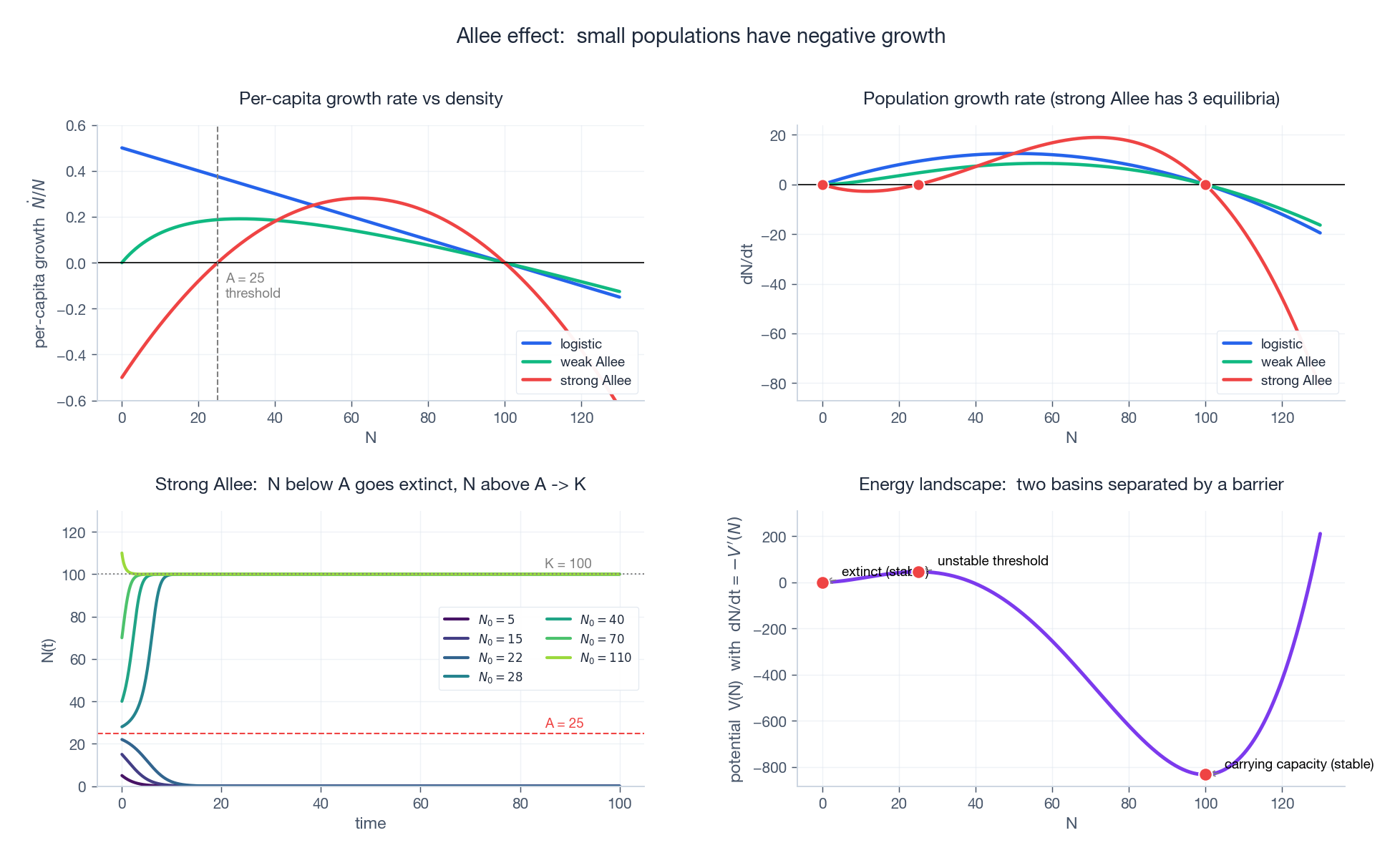
Top-left: per-capita growth rate $\dot N / N$ vs density. Logistic (blue) is positive everywhere up to $K$ . Strong Allee (red) is negative below the threshold $A$ . Top-right: $\dot N$ vs $N$ — strong Allee has three equilibria. Bottom-left: trajectories from various initial populations — those starting below $A$ collapse to extinction; those above $A$ rise to carrying capacity. Bottom-right: the corresponding “potential” $V(N)$ such that $\dot N = -V'(N)$ . The two stable states (extinction at $N = 0$ , carrying capacity at $N = K$ ) are valleys; the threshold $A$ is the barrier that separates them. A noise-perturbed system can tunnel between basins, providing a clean model of “regime shifts” in ecology.
Predator-Prey: Lotka-Volterra#
$$ \boxed{\;\dot x = \alpha x - \beta x y, \qquad \dot y = \delta x y - \gamma y.\;} $$- $\alpha$ : prey intrinsic growth (no predators)
- $\gamma$ : predator death rate (no prey)
- $\beta, \delta$ : encounter rates
Setting derivatives to zero gives two equilibria: extinction $(0, 0)$ — a saddle — and coexistence $(\gamma/\delta,\ \alpha/\beta)$ — a neutral centre.
A conserved quantity#
$$ H(x, y) = \delta x - \gamma\ln x + \beta y - \alpha\ln y. $$A direct calculation shows $\dot H = 0$ along solutions. So every Lotka-Volterra orbit lies on a level set of $H$ . The level sets are closed curves around the centre, which is why solutions are periodic (and why the centre is genuinely neutral, not stable).
This conservation is fragile: any small perturbation of the equations destroys it. Real ecosystems do not satisfy Lotka-Volterra exactly, so real cycles are typically limit cycles (under Holling responses below) rather than the LV continuum of cycles.
The hare-lynx data#
The Hudson Bay Company’s pelt records (1845-1930) show a beautiful 10-year cycle of snowshoe hare and Canada lynx. Lotka-Volterra qualitatively reproduces it. Quantitatively, ecologists now believe the lynx-hare cycle is actually driven by the hare-vegetation interaction, with lynx riding along, but the historical match was striking enough to make Lotka-Volterra famous.
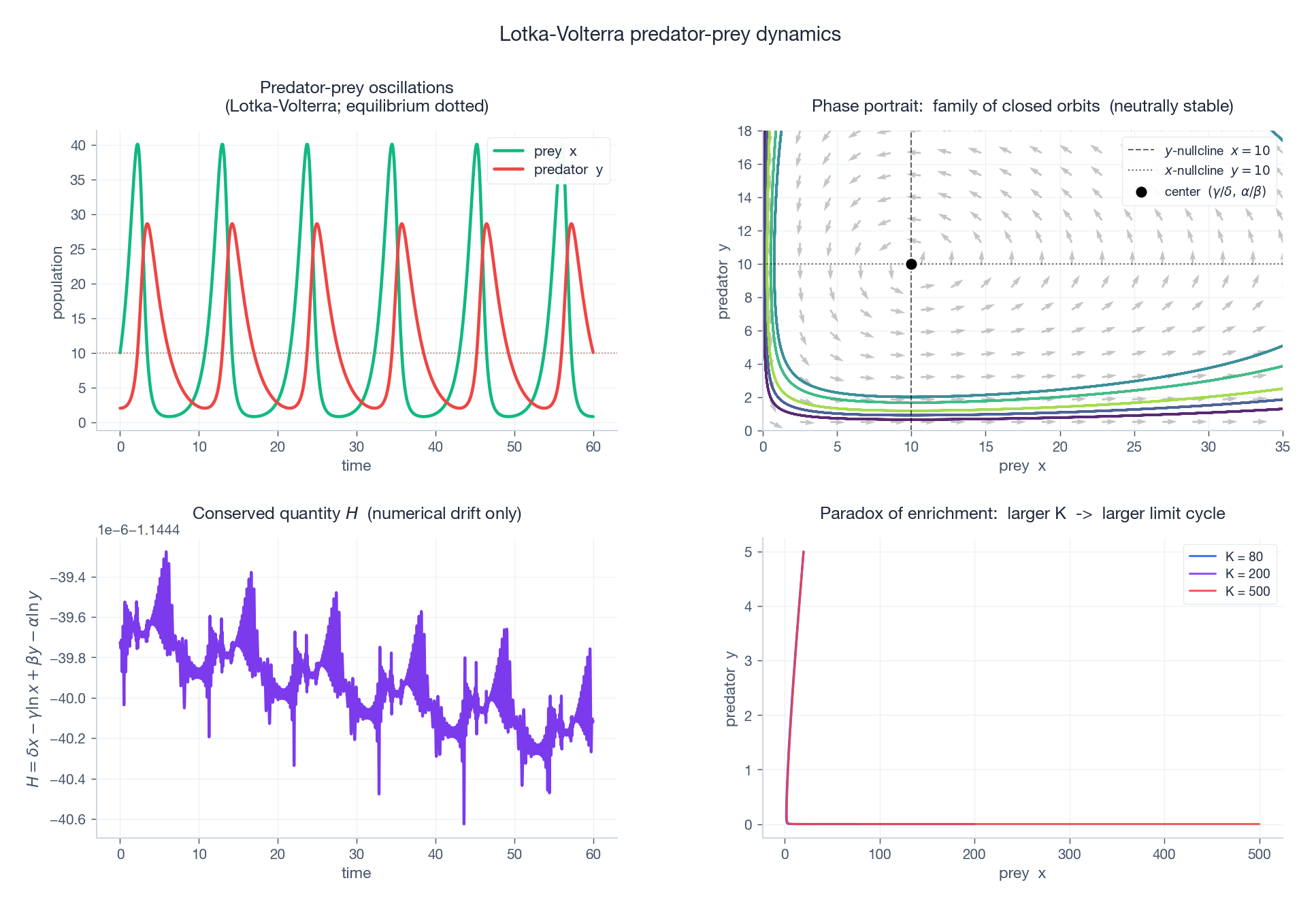
Top-left: the classic out-of-phase oscillation — prey peaks first, predator peaks a quarter cycle later. Top-right: phase plane with five different initial conditions tracing five different closed orbits, all centred on $(\gamma/\delta,\ \alpha/\beta)$ . Vector field shows the rotation direction. Bottom-left: $H$ along one orbit — numerical drift only (a real conservation law). Bottom-right: with a Holling Type II prey response and logistic prey growth, increasing the prey carrying capacity $K$ destabilises the equilibrium and produces a growing limit cycle — the paradox of enrichment.
| |
Functional responses (Holling)#
Real predators saturate — a wolf cannot eat infinitely many rabbits in a day. Holling categorised three responses:
- Type I: linear $g(x) = ax$ (Lotka-Volterra default; biologically rare).
- Type II: $g(x) = ax / (1 + ahx)$ — saturates at $1/h$ . Most common.
- Type III: $g(x) = ax^2 / (1 + ahx^2)$ — sigmoidal; allows prey switching at low density.
Replacing the LV interaction with a Holling-II response gives the Rosenzweig-MacArthur model, whose equilibrium can lose stability through a Hopf bifurcation as the prey carrying capacity grows. Higher $K$ means more food for prey, larger predator population, larger prey crashes, larger limit cycle, eventual extinction. More food is bad.
Paradox of enrichment#
The arithmetic: at fixed predator-prey parameters, the Hopf bifurcation occurs when $K$ crosses a threshold, after which a limit cycle appears whose amplitude grows like $\sqrt{K - K_c}$ . Eventually the cycle approaches the axes and any small noise drives a population to zero. This is not an idealised counter-intuition — it has been observed in lake-fish enrichment experiments.
Two-Species Competition#
$$ \dot N_1 = r_1 N_1\!\left(1 - \frac{N_1 + \alpha_{12} N_2}{K_1}\right), \qquad \dot N_2 = r_2 N_2\!\left(1 - \frac{N_2 + \alpha_{21} N_1}{K_2}\right). $$The dimensionless competition coefficients $\alpha_{ij}$ measure how much one individual of species $j$ depresses the per-capita growth of species $i$ , relative to one of its own.
The system has up to four equilibria:
- $(0, 0)$ — always unstable when both species can grow alone
- $(K_1, 0)$ — species 1 wins
- $(0, K_2)$ — species 2 wins
- interior $\bigl(\hat N_1, \hat N_2\bigr)$ if it exists — coexistence
Stability of these depends on whether each species can invade when the other is at carrying capacity. Comparing growth rates gives four canonical outcomes:
| Condition | Outcome |
|---|---|
| $\alpha_{12} < K_1/K_2$ AND $\alpha_{21} < K_2/K_1$ | Stable coexistence |
| $\alpha_{12} < K_1/K_2$ AND $\alpha_{21} > K_2/K_1$ | Species 1 wins |
| $\alpha_{12} > K_1/K_2$ AND $\alpha_{21} < K_2/K_1$ | Species 2 wins |
| $\alpha_{12} > K_1/K_2$ AND $\alpha_{21} > K_2/K_1$ | Bistable: founder effect |
The competitive exclusion principle (Gause 1934) is the corollary: two species with identical niches ($\alpha_{12} = \alpha_{21} = 1$ and $K_1 = K_2$ ) cannot stably coexist. Coexistence requires niche differentiation — intraspecific competition must exceed interspecific competition.
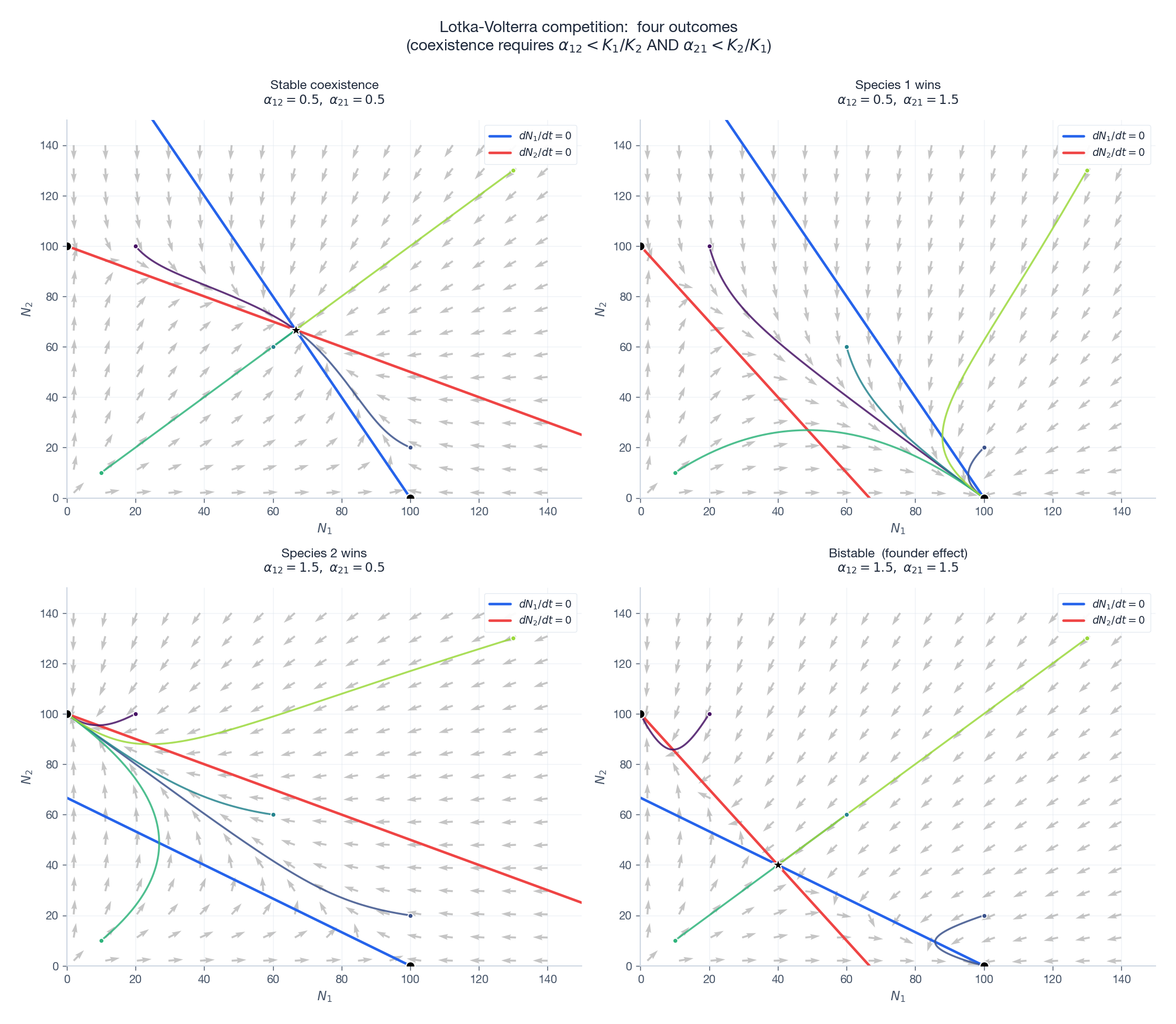
Each panel shows nullclines (blue / red lines), vector field (gray arrows), trajectories from five initial conditions (coloured), and equilibria (black dots / star). Top-left: coexistence — nullclines cross with the right orientation; the interior star is stable. Top-right and bottom-left: exclusion — the interior equilibrium does not exist, all trajectories funnel to one axis. Bottom-right: bistability — the interior equilibrium is a saddle, and the basin boundary is its stable manifold; whichever species starts in the right basin wins.
Age-Structured Models#
$$ \boxed{\;n_{t+1} = L\,n_t,\quad L = \begin{pmatrix} F_0 & F_1 & \cdots & F_m \\ P_0 & 0 & \cdots & 0 \\ 0 & P_1 & \cdots & 0 \\ \vdots & & \ddots & \vdots \\ 0 & 0 & P_{m-1} & 0 \end{pmatrix}.\;} $$- $F_i$ = age-$i$ fertility (offspring per timestep)
- $P_i$ = survival probability from age $i$ to age $i + 1$
This is just $n_{t+1} = L\,n_t$ ; the long-run dynamics is governed by the dominant eigenvalue $\lambda$ of $L$ :
- $\lambda > 1$ : geometric growth at rate $\lambda$
- $\lambda = 1$ : stable population
- $\lambda < 1$ : decline to extinction
The corresponding (right) eigenvector is the stable age distribution — the fraction of the population in each age class once the dynamics has equilibrated. Any initial distribution converges to it (up to a possibly oscillating phase if $L$ has complex eigenvalues of equal magnitude, which Perron-Frobenius rules out for non-negative irreducible Leslie matrices).
Why $\lambda$ is the number#
The net reproductive rate is $R_0 = \sum_i \ell_i F_i$ where $\ell_i = \prod_{j < i} P_j$ is survival to age $i$ . The relation $R_0 = 1 \Leftrightarrow \lambda = 1$ holds, and for population growth what matters is both how many offspring you produce and when (early offspring contribute to growth more, because they reproduce sooner). This timing effect is captured automatically by the eigenvalue.
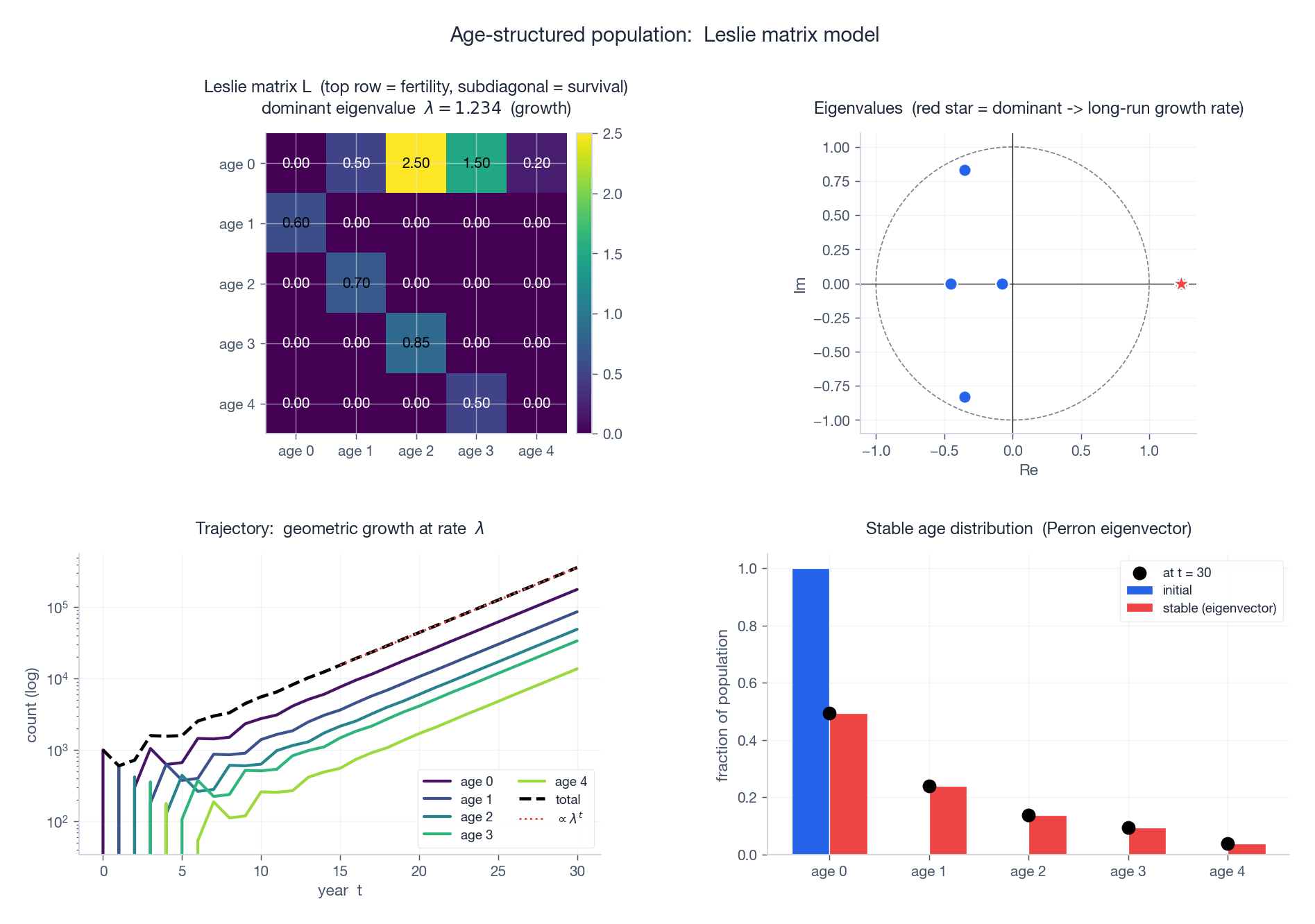
Top-left: Leslie matrix $L$ as a heatmap — top row holds fertilities $F_i$ , subdiagonal holds survivals $P_i$ . Top-right: eigenvalues in the complex plane; the dominant real eigenvalue (red star) sits outside the unit circle, so the population grows. Bottom-left: trajectory starting from 1000 newborns. Geometric growth at rate $\lambda$ takes hold within 10-15 years. Bottom-right: stable age distribution (Perron eigenvector, red bars) versus a trajectory snapshot at $t = 30$ (black dots) — they agree.
| |
Metapopulations: Many Patches#
$$ \boxed{\;\dot p = c\,p\,(1 - p) - e\,p,\;} $$where $p$ is the fraction occupied, $c$ is the colonisation rate (per occupied patch, into empty patches) and $e$ is the local extinction rate. The equilibrium is $p^* = 1 - e/c$ (positive iff $c > e$ ).
This is structurally identical to the SIS infection model, with patches as “individuals” and colonisation as “transmission”. The metapopulation persists iff $c > e$ — a regional extinction threshold.
The lesson for conservation: even if every individual habitat patch is healthy, regional extinction can occur if the colonisation rate (corridors, dispersal) is too low. Roads and fences fragment habitat by cutting $c$ , even if each fragment looks fine.
Spatial Spread: Fisher-KPP#

The proof, in two lines: linearise the leading edge ($N \ll K$ ); a travelling-wave ansatz $N = e^{-\lambda(x - ct)}$ requires $c = D\lambda + r/\lambda$ , minimised over $\lambda$ at $c_{\min} = 2\sqrt{Dr}$ . (The actual selected speed is the linear minimum — this is the celebrated KPP selection principle.)
This formula is everywhere in ecology: it predicts the speed of plant-range expansion under climate change, the muskrat invasion of Europe (literally measured at $\approx \sqrt{Dr}$ in the 1920s), and the wave speed of advantageous-allele fixation in genetics.
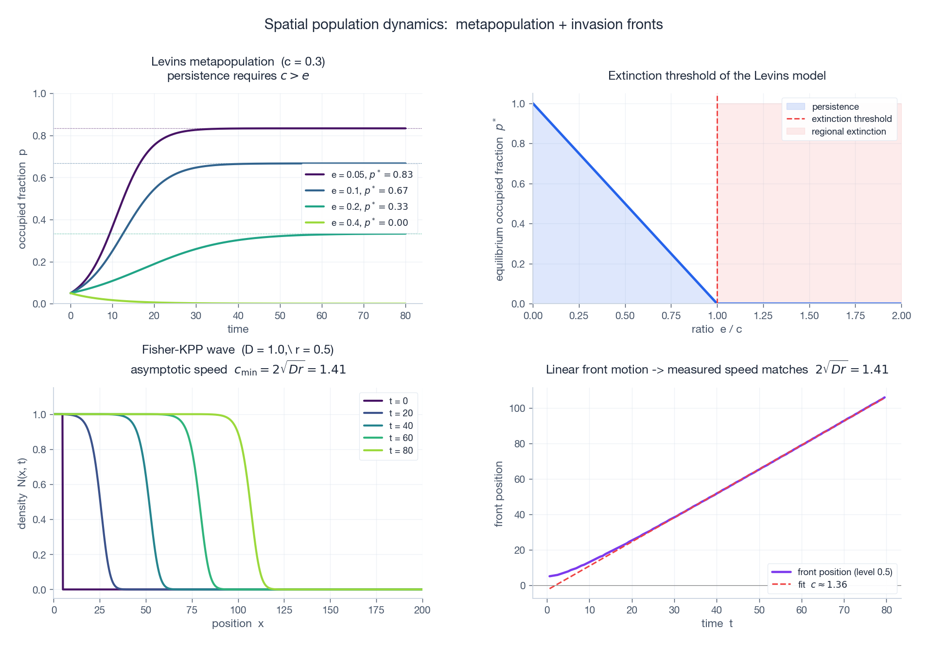
Top-left: Levins $p(t)$ for various extinction rates $e$ . Higher $e$ means lower $p^*$ ; if $e > c$ the metapopulation goes extinct regionally. Top-right: $p^*$ as a function of $e/c$ — the extinction threshold at $e = c$ . Bottom-left: Fisher-KPP traveling wave snapshots at $t = 0, 20, 40, 60, 80$ . The front is a smooth front of constant shape moving at speed $c_{\min} = 2\sqrt{Dr}$ . Bottom-right: numerically tracked front position; the slope of the linear fit matches $2\sqrt{Dr}$ to within 2%.
Beyond Fisher: Turing patterns#
When two species (e.g. activator and inhibitor, or predator and prey) diffuse at different rates, the homogeneous equilibrium can become unstable to spatial perturbations — spontaneous patterns form. This is the Turing instability (1952). The same mechanism is hypothesised to underlie animal coat patterns, vegetation stripes in semi-arid regions, and certain mussel-bed dynamics. It is the linchpin of mathematical morphogenesis.
Summary#
| Model | Equation | Key feature |
|---|---|---|
| Malthus | $\dot N = rN$ | unbounded exponential |
| Logistic | $\dot N = rN(1 - N/K)$ | saturation at $K$ |
| Allee (strong) | $\dot N = rN(1 - N/K)(N/A - 1)$ | extinction threshold $A$ , bistability |
| Lotka-Volterra | $\dot x = \alpha x - \beta xy,\ \dot y = \delta xy - \gamma y$ | conserved quantity, neutral cycles |
| Holling Type II | $g(x) = ax/(1 + ahx)$ | predator saturation, paradox of enrichment |
| LV competition | $\dot N_i = r_i N_i (1 - (N_i + \alpha_{ij} N_j)/K_i)$ | four canonical outcomes |
| Leslie | $n_{t+1} = L n_t$ | dominant eigenvalue = growth rate; stable age distribution |
| Levins | $\dot p = cp(1 - p) - ep$ | regional extinction threshold $e/c$ |
| Fisher-KPP | $\partial_t N = D\partial_x^2 N + rN(1 - N/K)$ | wave speed $2\sqrt{Dr}$ |
Mathematical ecology is small in number of equations but vast in number of behaviours. A handful of compositional rules — diffusion + reaction, single-species + age structure, mean-field + heterogeneity — generate the entire field.
Exercises#
Conceptual.
- Starting from the strong-Allee equation, derive the potential $V(N)$ explicitly and identify the locations of the two basins and the barrier.
- Why is the Lotka-Volterra centre neutral and not asymptotically stable? Use the conserved quantity to argue.
- Two competitors satisfy $\alpha_{12} = 0.9, \alpha_{21} = 0.9$ , $K_1 = K_2 = 100$ , $r_1 = r_2 = 0.5$ . Compute the interior equilibrium and decide its stability.
Computational.
- Verify the analytical formula $c_{\min} = 2\sqrt{Dr}$ for the Fisher-KPP wave by simulating with a fine mesh and tracking the 50%-density level.
- Vary $K$ in the Rosenzweig-MacArthur model and find the Hopf bifurcation point numerically. Compare to the analytical prediction.
- Construct a Leslie matrix for a species with $F = (0, 0, 1.2, 1.0, 0.4)$ , $P = (0.7, 0.85, 0.85, 0.5)$ . What is the long-run growth rate? Stable age distribution?
Programming.
- Animate the bistable-competition phase plane: vary the initial condition continuously across the saddle’s stable manifold and watch the basin switch.
- Implement a stochastic Levins model on $1000$ patches with rates $c, e$ . Compare its mean fraction occupied to the deterministic $p^* = 1 - e/c$ as $e/c$ approaches 1.
- Build a 2D Fisher-KPP simulator and watch the wave from a localised initial condition. Compare with the 1D wave speed.
- Implement the Leslie model with a time-varying fertility $F_i(t)$ representing seasonal cycles; observe how the population structure tracks the forcing.
References#
- Murray, Mathematical Biology I & II, Springer (2002, 2003)
- Edelstein-Keshet, Mathematical Models in Biology, SIAM Classic (2005)
- Kot, Elements of Mathematical Ecology, Cambridge (2001)
- Hastings, Population Biology: Concepts and Models, Springer (1997)
- Lotka, Elements of Physical Biology, Williams & Wilkins (1925)
- Volterra, “Variazioni e fluttuazioni del numero d’individui in specie animali conviventi,” Mem. R. Acad. Naz. dei Lincei (1926)
- Fisher, “The wave of advance of advantageous genes,” Ann. Eugenics 7 (1937)
- Hanski, Metapopulation Ecology, Oxford (1999)
- Turing, “The chemical basis of morphogenesis,” Phil. Trans. Roy. Soc. B 237 (1952)
ODE Foundations 18 parts
- 01 Ordinary Differential Equations (1): Origins and Intuition
- 02 Ordinary Differential Equations (2): First-Order Methods
- 03 Ordinary Differential Equations (3): Higher-Order Linear Theory
- 04 Ordinary Differential Equations (4): The Laplace Transform
- 05 Ordinary Differential Equations (5): Power Series and Special Functions
- 06 Ordinary Differential Equations (6): Linear Systems and the Matrix Exponential
- 07 Ordinary Differential Equations (7): Stability Theory
- 08 Ordinary Differential Equations (8): Nonlinear Systems and Phase Portraits
- 09 Ordinary Differential Equations (9): Chaos Theory and the Lorenz System
- 10 Ordinary Differential Equations (10): Bifurcation Theory
- 11 Ordinary Differential Equations (11): Numerical Methods
- 12 Ordinary Differential Equations (12): Boundary Value Problems
- 13 Ordinary Differential Equations (13): Introduction to Partial Differential Equations
- 14 Ordinary Differential Equations (14): Epidemic Models and Epidemiology
- 15 Ordinary Differential Equations (15): Population Dynamics you are here
- 16 Ordinary Differential Equations (16): Fundamentals of Control Theory
- 17 Ordinary Differential Equations (17): Physics and Engineering Applications
- 18 Ordinary Differential Equations (18): Frontiers and Series Finale