Recommendation Systems (9): Multi-Task Learning and Multi-Objective Optimization

A live e-commerce ranker doesn’t optimize just one number. The same model that decides which product to show you also predicts, in the same forward pass, whether you will click, add it to your cart, pay for it, return it, or leave a positive review. Each prediction is a different task with its own data distribution, scarcity, and incentives. These tasks are tightly coupled: a clicker is more likely to convert, a converter is more likely to write a review, and a high-CTR thumbnail can attract clicks that reduce watch time.

Multi-task learning (MTL) is how production systems handle this. Instead of training one model per objective and stitching scores together, we train one neural network with several output heads and let the shared trunk learn representations that serve all of them at once. The hard part is not the architecture diagram — it is making sure the heads cooperate instead of fighting over the shared weights.

This post provides the mental model and working code for the four architectures you’ll encounter in industry: Shared-Bottom, ESMM, MMoE, PLE. It also explains why the simple version fails (negative transfer, gradient conflict, sample selection bias) and how Uncertainty Weighting, GradNorm, and Pareto trade-offs address these issues.

What You Will Learn#

Why ranking is inherently multi-objective and what goes wrong when you ignore that
Sample selection bias in CVR prediction and ESMM’s chain-rule fix
Four architectures — Shared-Bottom, ESMM, MMoE, PLE — and when each one wins
Loss balancing: Uncertainty Weighting, GradNorm, Pareto frontiers
A complete PyTorch training loop that you can lift into a project

Prerequisites#

PyTorch basics (modules, forward pass, loss functions)
CTR prediction concepts (Part 4 )
Embedding layers (Part 5 )

Why Recommenders Are Multi-Objective#

Optimizing One Number Is the Wrong Game#

Picture a restaurant recommender. If you only optimize clicks, the model learns that lurid food photos and clickbait names work great, but your conversion rate plummets. If you only optimize bookings, you surface safe national chains with no room for discovery. If you only optimize stars, you push fancy, expensive places that few people book. The honest objective is a bundle:

Will the user click? (engagement)
Will they actually visit? (conversion)
Will they enjoy it? (satisfaction)
Will they come back? (retention)

The same pattern shows up everywhere:

Domain	Typical objectives
E-commerce	CTR, CVR, revenue per impression, return rate, review quality
Short video	CTR, watch time, like/share rate, follow rate
Ads	CTR, CVR, cost per acquisition, lifetime value

These metrics are correlated but distinct. The job of an MTL model is to exploit the correlation (clicks inform the conversion head about user intent) without letting one objective dominate.

Sample Selection Bias: Why Naive CVR Is Broken#

Here is the subtle problem that motivated ESMM. Suppose you want a conversion model: given a user and an item, what is $P(\text{buy} \mid \text{shown})$ ?

Training labels exist only on clicked items — you can only observe a buy after a click.
At serving time the model must score every candidate, including items the user never clicked.

You train on the slice of impressions that were clicked, then deploy on all impressions. This is sample selection bias: a textbook covariate shift between training and serving.

P(\text{buy} \mid \text{imp}) = P(\text{click} \mid \text{imp}) \cdot P(\text{buy} \mid \text{click})

Read it in English: “the probability of buying after seeing an item equals the probability of clicking it times the probability of buying given that you clicked.” The first factor (CTR) and the product (CTCVR) are both observable on the whole impression space. So we train those two and let CVR fall out as a free byproduct — no biased slice required.

What MTL Buys You (and What It Costs)#

Wins

Data efficiency. Sparse tasks (purchases, follows) piggyback on dense tasks (impressions, clicks).
Implicit regularization. Sharing weights across tasks discourages overfitting to any single label.
Cheaper serving. One forward pass produces every score the ranker needs.
Better generalization. Joint training tends to find representations that generalize beyond any single objective.

Costs

Negative transfer. Tasks can pull shared weights in opposite directions and make every head worse than its single-task baseline.
Loss balancing. CTR loss may sit around 0.3 while a revenue MSE sits at 100 — naive sums let one task drown the others.
Architecture choices. You have to decide what to share and what to keep private, with surprisingly little theory to guide you.

The architectures below are essentially four answers to the same question: how much and where to share?

Architecture 1: Shared-Bottom#

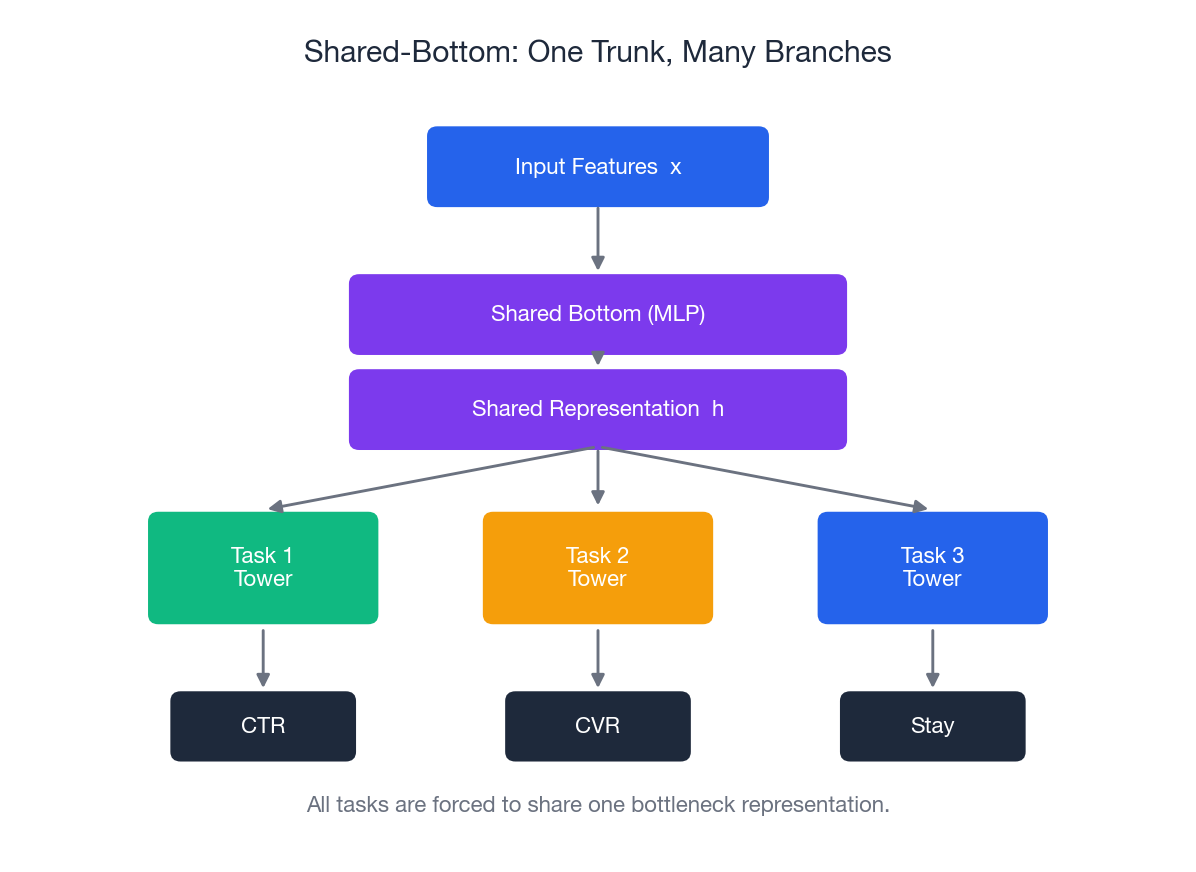
Shared-Bottom architecture: one shared MLP feeds three independent task towers

h = f_{\text{shared}}(x), \qquad \hat{y}_k = f_k(h), \quad k=1,\dots,K

Every task sees the same $$h$$ . That is the single design assumption — and the single failure mode.

Implementation#

 1
 2
 3
 4
 5
 6
 7
 8
 9
10
11
12
13
14
15
16
17
18
19
20
21
22
23
24
25
26
27
28
29
30
31
32
33
34
35
36
37
38
39
40
41
42
43
44
45
46
47
48
49
50
51
52
53
54
import torch
import torch.nn as nn
import torch.nn.functional as F

class SharedBottomMTL(nn.Module):
    """Shared-Bottom MTL: one trunk, K task-specific towers.

    Works well when tasks are aligned. Breaks down (negative transfer)
    when tasks pull the shared trunk in opposite directions.
    """

    def __init__(self, input_dim, shared_hidden_dims, task_hidden_dims,
                 num_tasks, task_types):
        super().__init__()
        self.num_tasks = num_tasks
        self.task_types = task_types

        # ---- shared trunk
        shared, prev = [], input_dim
        for h in shared_hidden_dims:
            shared += [nn.Linear(prev, h), nn.BatchNorm1d(h),
                       nn.ReLU(), nn.Dropout(0.2)]
            prev = h
        self.shared_bottom = nn.Sequential(*shared)

        # ---- one tower per task
        self.task_towers = nn.ModuleList()
        for k in range(num_tasks):
            layers, prev = [], shared_hidden_dims[-1]
            for h in task_hidden_dims:
                layers += [nn.Linear(prev, h), nn.BatchNorm1d(h),
                           nn.ReLU(), nn.Dropout(0.1)]
                prev = h
            layers.append(nn.Linear(prev, 1))
            if task_types[k] == 'binary':
                layers.append(nn.Sigmoid())
            self.task_towers.append(nn.Sequential(*layers))

    def forward(self, x):
        h = self.shared_bottom(x)
        return [tower(h) for tower in self.task_towers]

# 3 tasks: CTR (binary), CVR (binary), Revenue (regression)
model = SharedBottomMTL(
    input_dim=128,
    shared_hidden_dims=[256, 128, 64],
    task_hidden_dims=[32, 16],
    num_tasks=3,
    task_types=['binary', 'binary', 'regression'],
)

x = torch.randn(32, 128)
ctr, cvr, rev = model(x)
print(ctr.shape, cvr.shape, rev.shape)  # all (32, 1)

Why It Eventually Hurts#

If two tasks disagree on what the shared representation should encode—e.g., CTR rewards eye-catching novelty while CVR rewards reliable signals—the trunk must compromise. This compromise often makes both tasks perform worse than their single-task baselines. This is negative transfer, and it’s the reason for the other architectures below.

Architecture 2: ESMM (Entire Space Multi-Task Model)#

ESMM was Alibaba’s answer to sample selection bias in CVR. The architecture itself is small. The trick is what gets supervised, and where.

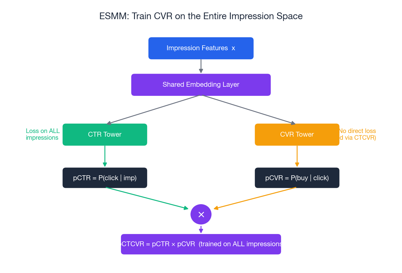
ESMM architecture: shared embedding feeds CTR and CVR towers; CTCVR is the product, supervised on all impressions

The Idea#

Don’t train CVR directly on the clicked-only slice. Train two things on the full impression space:

pCTR = $P(\text{click} \mid \text{imp})$ , supervised by the click label
pCTCVR = $P(\text{click and buy} \mid \text{imp})$ , supervised by click AND buy

CVR is then defined implicitly: $\text{pCTCVR} = \text{pCTR} \times \text{pCVR}$ . Backprop through the multiplication shapes the CVR tower without ever asking it to fit a biased label.

Implementation#

 1
 2
 3
 4
 5
 6
 7
 8
 9
10
11
12
13
14
15
16
17
18
19
20
21
22
23
24
25
26
27
28
29
30
31
32
33
34
35
36
37
38
39
40
41
42
43
44
45
46
47
48
49
50
51
52
53
54
55
56
class ESMM(nn.Module):
    """Entire-Space Multi-Task Model.

    Decompose P(buy|imp) = P(click|imp) * P(buy|click).
    Train CTR and CTCVR on every impression; CVR is supervised
    *implicitly* through the product. No more selection bias.
    """

    def __init__(self, input_dim, hidden_dims):
        super().__init__()
        self.embedding = nn.Sequential(
            nn.Linear(input_dim, hidden_dims[0]),
            nn.ReLU(), nn.Dropout(0.2),
        )
        self.ctr_tower = self._tower(hidden_dims)
        self.cvr_tower = self._tower(hidden_dims)

    def _tower(self, dims):
        layers, prev = [], dims[0]
        for h in dims[1:]:
            layers += [nn.Linear(prev, h), nn.ReLU(), nn.Dropout(0.2)]
            prev = h
        layers += [nn.Linear(prev, 1), nn.Sigmoid()]
        return nn.Sequential(*layers)

    def forward(self, x):
        h = self.embedding(x)
        pctr = self.ctr_tower(h)            # P(click | imp)
        pcvr = self.cvr_tower(h)            # P(buy | click)
        pctcvr = pctr * pcvr                # P(click AND buy | imp)
        return pctr, pcvr, pctcvr

def esmm_loss(pctr, pcvr, pctcvr, click_label, buy_label):
    """ESMM loss.

    - CTR loss on the FULL batch (every impression has a click label).
    - CTCVR loss on the FULL batch (click AND buy is observable for all).
    - CVR has NO direct loss -- gradient flows in through the product.
    """
    ctcvr_label = click_label * buy_label  # 1 only if clicked AND bought
    loss_ctr = F.binary_cross_entropy(pctr, click_label.float())
    loss_ctcvr = F.binary_cross_entropy(pctcvr, ctcvr_label.float())
    return loss_ctr + loss_ctcvr

# Mini training step
model = ESMM(input_dim=128, hidden_dims=[256, 128, 64])
opt = torch.optim.Adam(model.parameters(), lr=1e-3)

x = torch.randn(32, 128)
click = torch.randint(0, 2, (32, 1)).float()
buy = torch.randint(0, 2, (32, 1)).float()  # only meaningful where click=1

pctr, pcvr, pctcvr = model(x)
loss = esmm_loss(pctr, pcvr, pctcvr, click, buy)
loss.backward(); opt.step()
print(f"loss = {loss.item():.4f}")

Why It Works#

No biased slice. CTR and CTCVR live on every impression. CVR is never asked to fit a label that exists only after clicking.
Mathematical consistency. By construction $\text{pCTCVR} = \text{pCTR} \times \text{pCVR}$ , so the three scores you serve cannot contradict each other.
Cheap to deploy. It is the same shape as a Shared-Bottom with two binary heads. Production ranking pipelines barely notice.

In Alibaba’s original paper this trick lifted CVR AUC by about 2-3% on Taobao. That is a lot for a one-line architectural change.

Architecture 3: MMoE (Multi-gate Mixture-of-Experts)#

Shared-Bottom forces every task through one bottleneck. MMoE keeps a pool of expert sub-networks and lets each task softly choose its own mixture of experts.

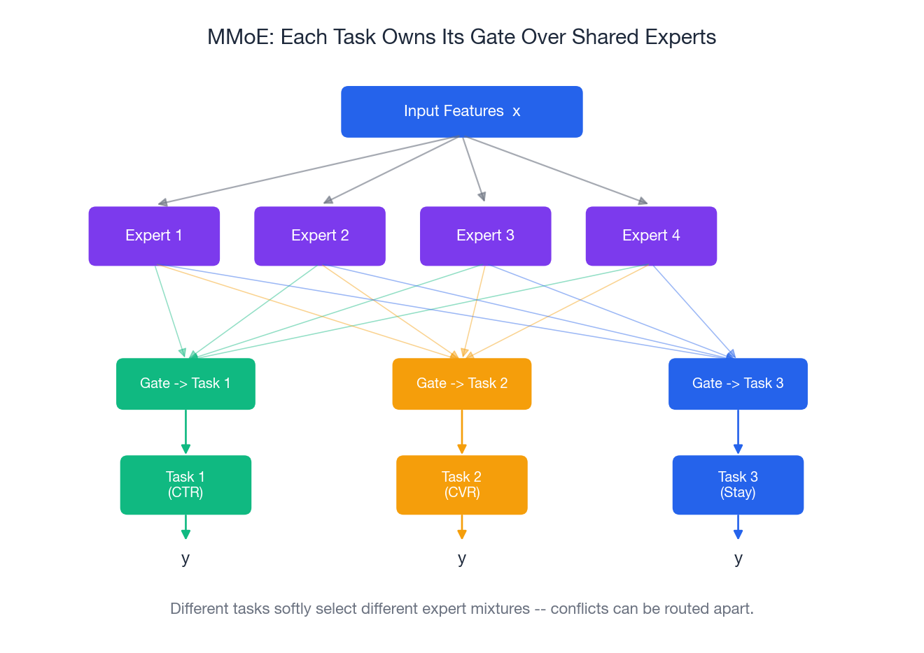
MMoE architecture: a pool of expert MLPs and one gating network per task

The Analogy#

You are organizing a dinner party with three jobs: cooking, decor, music. Instead of hiring one person to do all three (Shared-Bottom), you hire four specialists. Each job has its own manager (gate) who decides how much weight to give each specialist. The cooking manager leans on the chef and the sommelier; the decor manager leans on the florist and the lighting designer. The chef may still throw in a plating idea for decor — managers are free to mix.

The Math#

f_k(x) = \sum_{i=1}^{n} g_k^{(i)}(x) \cdot E_i(x), \qquad g_k(x) = \mathrm{softmax}(W_k x)

Each gate is just a tiny linear-then-softmax network. Conflicting tasks learn to point at different experts; cooperative tasks learn to share.

Implementation#

 1
 2
 3
 4
 5
 6
 7
 8
 9
10
11
12
13
14
15
16
17
18
19
20
21
22
23
24
25
26
27
28
29
30
31
32
33
34
35
36
37
38
39
40
41
42
43
44
45
46
47
48
49
50
51
52
53
54
55
56
57
58
59
60
61
62
63
64
65
66
67
class Expert(nn.Module):
    def __init__(self, input_dim, hidden_dim, output_dim):
        super().__init__()
        self.net = nn.Sequential(
            nn.Linear(input_dim, hidden_dim), nn.ReLU(), nn.Dropout(0.1),
            nn.Linear(hidden_dim, output_dim), nn.ReLU(),
        )

    def forward(self, x):
        return self.net(x)

class MMoE(nn.Module):
    """Multi-gate Mixture-of-Experts.

    A pool of n experts; each of the K tasks has its own gate that
    forms a soft mixture over them. Conflicting tasks can route to
    different experts -- the model decides.
    """

    def __init__(self, input_dim, num_experts, expert_hidden_dim,
                 expert_output_dim, num_tasks, task_hidden_dims, task_types):
        super().__init__()
        self.num_tasks = num_tasks

        self.experts = nn.ModuleList([
            Expert(input_dim, expert_hidden_dim, expert_output_dim)
            for _ in range(num_experts)
        ])
        self.gates = nn.ModuleList([
            nn.Sequential(nn.Linear(input_dim, num_experts), nn.Softmax(dim=1))
            for _ in range(num_tasks)
        ])

        self.task_towers = nn.ModuleList()
        for k in range(num_tasks):
            layers, prev = [], expert_output_dim
            for h in task_hidden_dims:
                layers += [nn.Linear(prev, h), nn.ReLU(), nn.Dropout(0.1)]
                prev = h
            layers.append(nn.Linear(prev, 1))
            if task_types[k] == 'binary':
                layers.append(nn.Sigmoid())
            self.task_towers.append(nn.Sequential(*layers))

    def forward(self, x):
        # All experts in one stacked tensor: (B, n_experts, expert_dim)
        E = torch.stack([e(x) for e in self.experts], dim=1)

        outputs, gates_out = [], []
        for k in range(self.num_tasks):
            w = self.gates[k](x)               # (B, n_experts)
            gates_out.append(w)
            mix = (w.unsqueeze(2) * E).sum(1)  # (B, expert_dim)
            outputs.append(self.task_towers[k](mix))
        return outputs, gates_out

model = MMoE(
    input_dim=128, num_experts=4, expert_hidden_dim=64,
    expert_output_dim=32, num_tasks=3, task_hidden_dims=[16],
    task_types=['binary', 'binary', 'regression'],
)
x = torch.randn(32, 128)
outs, gates = model(x)

# Inspect routing -- often Task 1 favors a different subset than Task 3
print("Task 1 gate weights:", gates[0][0].detach().round(decimals=2))
print("Task 3 gate weights:", gates[2][0].detach().round(decimals=2))

When MMoE Helps#

You suspect some tasks conflict but you don’t know which.
You want a single architecture that gracefully handles both cooperative and antagonistic mixes.
The gate weights themselves are useful telemetry — you can plot them and see which tasks share which experts.

Architecture 4: PLE (Progressive Layered Extraction)#

PLE, from Tencent, addresses an MMoE failure mode: even with gates, a shared expert pool can let one task’s gradients corrupt features another task depends on — the famous seesaw phenomenon where lifting CTR drops watch time by exactly the amount you lifted.

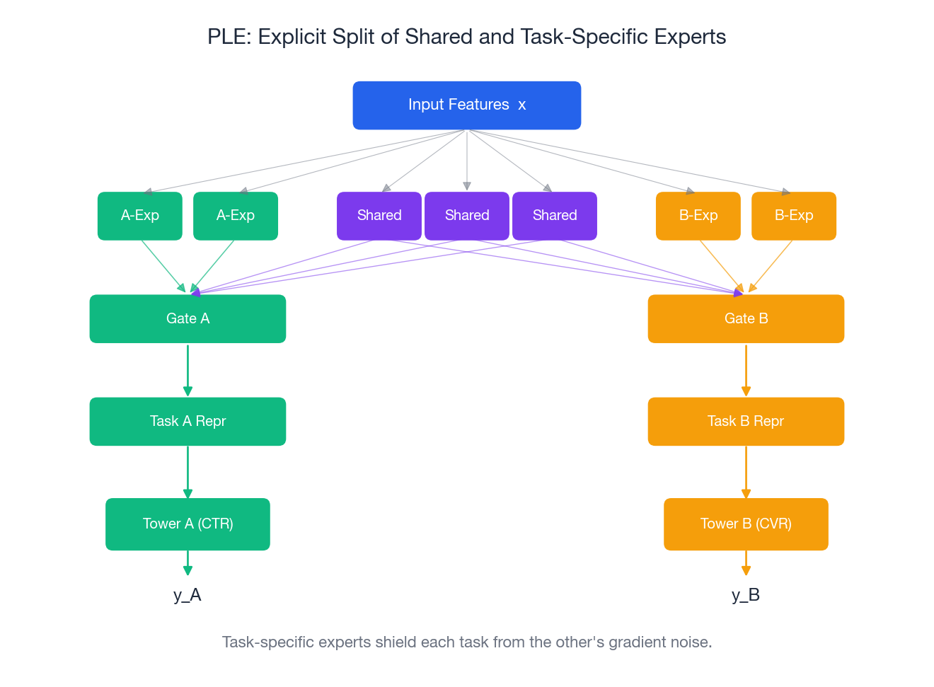
PLE architecture: shared experts plus task-specific experts, combined per task by a gate

The Idea#

Make the split explicit. Each task layer has:

Shared experts — visible to every task, learn cross-task patterns.
Task-specific experts — private to one task, never see another task’s gradient.

Each task’s gate combines shared experts with its own task-specific experts. Stack a couple of these layers and you get progressive extraction: lower layers do generic feature work, higher layers do task-specific refinement.

Implementation#

 1
 2
 3
 4
 5
 6
 7
 8
 9
10
11
12
13
14
15
16
17
18
19
20
21
22
23
24
25
26
27
28
29
30
31
32
33
34
35
36
37
38
39
40
41
42
43
44
45
46
47
48
49
50
51
52
53
54
55
56
57
58
59
60
61
62
63
64
65
66
67
68
69
70
71
72
73
74
75
76
77
78
79
class PLELayer(nn.Module):
    """One PLE block: shared experts + per-task experts + per-task gates."""

    def __init__(self, input_dim, num_shared, num_per_task,
                 expert_hidden, expert_out, num_tasks):
        super().__init__()
        self.num_tasks = num_tasks
        self.shared_experts = nn.ModuleList([
            Expert(input_dim, expert_hidden, expert_out)
            for _ in range(num_shared)
        ])
        self.task_experts = nn.ModuleList([
            nn.ModuleList([
                Expert(input_dim, expert_hidden, expert_out)
                for _ in range(num_per_task)
            ])
            for _ in range(num_tasks)
        ])
        total = num_shared + num_per_task
        self.gates = nn.ModuleList([
            nn.Sequential(nn.Linear(input_dim, total), nn.Softmax(dim=1))
            for _ in range(num_tasks)
        ])

    def forward(self, x):
        shared = torch.stack([e(x) for e in self.shared_experts], dim=1)
        out = []
        for k in range(self.num_tasks):
            task_e = torch.stack([e(x) for e in self.task_experts[k]], dim=1)
            pool = torch.cat([shared, task_e], dim=1)
            w = self.gates[k](x).unsqueeze(2)
            out.append((w * pool).sum(1))
        return out

class PLE(nn.Module):
    """Progressive Layered Extraction with task-specific + shared experts."""

    def __init__(self, input_dim, num_layers, num_shared, num_per_task,
                 expert_hidden, expert_out, num_tasks,
                 task_hidden_dims, task_types):
        super().__init__()
        self.num_tasks = num_tasks
        self.layers = nn.ModuleList()
        prev = input_dim
        for _ in range(num_layers):
            self.layers.append(PLELayer(
                prev, num_shared, num_per_task,
                expert_hidden, expert_out, num_tasks,
            ))
            prev = expert_out

        self.task_towers = nn.ModuleList()
        for k in range(num_tasks):
            layers, p = [], expert_out
            for h in task_hidden_dims:
                layers += [nn.Linear(p, h), nn.ReLU(), nn.Dropout(0.1)]
                p = h
            layers.append(nn.Linear(p, 1))
            if task_types[k] == 'binary':
                layers.append(nn.Sigmoid())
            self.task_towers.append(nn.Sequential(*layers))

    def forward(self, x):
        # Each task carries its own representation through the stack.
        reps = [x] * self.num_tasks
        for layer in self.layers:
            # Each task feeds its own current representation into the next layer.
            reps = [layer(reps[k])[k] for k in range(self.num_tasks)]
        return [self.task_towers[k](reps[k]) for k in range(self.num_tasks)]

model = PLE(
    input_dim=128, num_layers=2,
    num_shared=2, num_per_task=2,
    expert_hidden=64, expert_out=32,
    num_tasks=3, task_hidden_dims=[16],
    task_types=['binary', 'binary', 'regression'],
)
out = model(torch.randn(32, 128))
print([o.shape for o in out])

Why The Split Matters#

A task-specific expert receives gradient only from its task. So when CTR’s gradient yanks the model in a direction CVR hates, the damage is confined to the shared experts — CVR’s private experts are untouched. In Tencent’s reported video-recommendation numbers PLE bought another ~0.4% AUC over MMoE on multiple engagement metrics, and meaningfully reduced the seesaw effect.

Picking an Architecture#

Situation	Pick	Reason
Tasks closely aligned, limited eng resources	Shared-Bottom	Simple, fast, good baseline
CVR prediction with clicked-only labels	ESMM	Removes selection bias by construction
Mix of related and possibly conflicting tasks	MMoE	Gates discover the right routing
Known mix of shared and conflicting patterns	PLE	Hard split caps negative transfer

A reasonable progression in a real project: ship Shared-Bottom; if any single-task baseline beats your MTL model on its own task, move to MMoE; if you observe seesaw, move to PLE.

Loss Balancing: Stop One Task From Eating The Others#

CTR loss might sit around 0.3, CVR around 0.05, a revenue MSE around 100. If you sum them, the regression task drowns the others. Balancing is not a finishing touch — it is the difference between the model learning two tasks and learning one and a half.

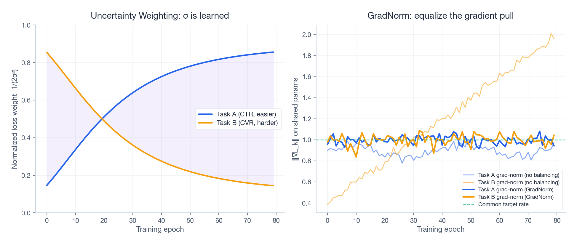
Uncertainty Weighting (Kendall et al., 2018)#

\mathcal{L}_{\text{total}} = \sum_k \frac{1}{2\sigma_k^2}\, \mathcal{L}_k + \log \sigma_k

Hard tasks naturally inflate $\sigma_k$ , which down-weights them; the $\log \sigma_k$ term stops $\sigma_k$ from running off to infinity. The picture is what you’d hope for — the easy task’s normalized weight grows as the hard task’s shrinks:

 1
 2
 3
 4
 5
 6
 7
 8
 9
10
11
12
13
class UncertaintyWeighting(nn.Module):
    """Learn per-task log-variance; downweight hard tasks automatically."""

    def __init__(self, num_tasks):
        super().__init__()
        self.log_var = nn.Parameter(torch.zeros(num_tasks))  # = 2 log sigma

    def forward(self, task_losses):
        total = 0.0
        for k, loss in enumerate(task_losses):
            precision = torch.exp(-self.log_var[k])  # 1 / sigma^2
            total = total + 0.5 * precision * loss + 0.5 * self.log_var[k]
        return total

GradNorm#

Uncertainty Weighting balances losses. GradNorm balances gradient magnitudes on the shared trunk. The intuition: a task whose gradient norm dwarfs the others is, mechanically, the one steering the trunk. GradNorm scales each task’s weight so that all tasks contribute roughly equal pull, with an optional bias toward tasks that are learning more slowly. The right panel above shows the raw norms drifting apart and being pulled back to a common rate.

Pareto Optimization#

When tasks genuinely conflict, no single weighting is “best” — only different trade-offs. Plotting the achievable (CTR-AUC, CVR-AUC) pairs gives you a Pareto frontier: solutions where you cannot improve one metric without sacrificing the other.

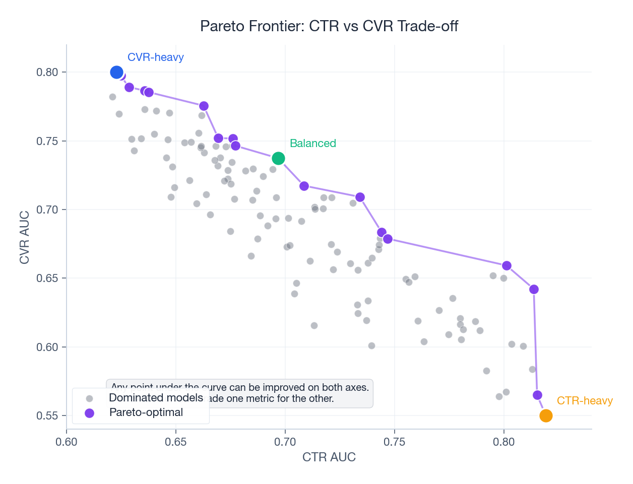
Pareto frontier between CTR AUC and CVR AUC, with three named operating points

In production this is less of a math problem and more of a product call: where on the curve does the business want to sit?

Why Tasks Fight: Gradient Conflict Up Close#

Why does any of this matter? Because shared parameters get pulled in two different directions at once. Pick a single shared weight $\theta$ ; task A says “increase me” and task B says “decrease me”. The joint update is the sum of two opposing arrows — often a much smaller step than either task wanted, in a direction neither task likes.

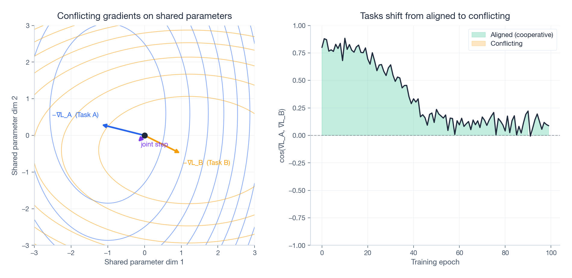
Two task gradients on shared parameters can point in conflicting directions; cosine similarity between gradients can flip negative during training

The right panel is the diagnostic you actually want in production: track the cosine similarity of the two tasks’ gradients on the shared trunk over training. If it slides negative and stays there, your model is in active gradient war. That is the precise moment to consider PLE (split the experts) or PCGrad (project away the conflicting component before stepping). Watching this number is cheap and tells you more than aggregate loss curves.

Industrial Reference Points#

Company	Architecture	Setting	Reported lift
Alibaba	ESMM	Taobao CVR	~2-3% AUC over biased CVR baseline
Google	MMoE	YouTube ranking	Significant improvement over Shared-Bottom across multiple objectives
Tencent	PLE	Tencent Video	~0.4% AUC over MMoE; seesaw effect reduced

Numbers are from the original papers; production systems iterate further.

A Complete Training Pipeline#

Putting MMoE together with Uncertainty Weighting and a real-feeling training loop:

 1
 2
 3
 4
 5
 6
 7
 8
 9
10
11
12
13
14
15
16
17
18
19
20
21
22
23
24
25
26
27
28
29
30
31
32
33
34
35
36
37
38
39
40
41
42
43
44
45
46
47
48
49
50
51
52
53
54
55
56
57
58
59
60
61
62
63
64
65
66
67
68
import torch
import torch.nn as nn
import torch.optim as optim
import torch.nn.functional as F
from torch.utils.data import Dataset, DataLoader
import numpy as np

class RecDataset(Dataset):
    def __init__(self, features, labels):
        self.x = torch.FloatTensor(features)
        self.y = {k: torch.FloatTensor(v) for k, v in labels.items()}
        self.tasks = list(labels.keys())

    def __len__(self):
        return len(self.x)

    def __getitem__(self, i):
        return {'x': self.x[i], **{t: self.y[t][i] for t in self.tasks}}

def train_epoch(model, loader, opt, balancer, tasks, device):
    model.train()
    running = {t: 0.0 for t in tasks}
    total = 0.0
    for batch in loader:
        x = batch['x'].to(device)
        y = {t: batch[t].to(device) for t in tasks}

        outs, _ = model(x)

        losses = []
        for k, t in enumerate(tasks):
            if t in ('ctr', 'cvr'):
                losses.append(F.binary_cross_entropy(outs[k].squeeze(), y[t]))
            else:
                losses.append(F.mse_loss(outs[k].squeeze(), y[t]))
            running[t] += losses[-1].item()

        loss = balancer(losses) if balancer else sum(losses)
        opt.zero_grad(); loss.backward(); opt.step()
        total += loss.item()

    n = len(loader)
    return total / n, {t: v / n for t, v in running.items()}

# ------ run it
N = 10_000
features = np.random.randn(N, 128).astype(np.float32)
labels = {
    'ctr': np.random.randint(0, 2, N).astype(np.float32),
    'cvr': np.random.randint(0, 2, N).astype(np.float32),
    'revenue': (np.random.rand(N) * 100).astype(np.float32),
}
loader = DataLoader(RecDataset(features, labels), batch_size=64, shuffle=True)

model = MMoE(
    input_dim=128, num_experts=4, expert_hidden_dim=64,
    expert_output_dim=32, num_tasks=3, task_hidden_dims=[16],
    task_types=['binary', 'binary', 'regression'],
)
balancer = UncertaintyWeighting(num_tasks=3)
opt = optim.Adam(list(model.parameters()) + list(balancer.parameters()), lr=1e-3)

for epoch in range(5):
    loss, per_task = train_epoch(model, loader, opt, balancer,
                                 ['ctr', 'cvr', 'revenue'], 'cpu')
    print(f"epoch {epoch+1}: loss={loss:.4f} | "
          f"ctr={per_task['ctr']:.4f} | cvr={per_task['cvr']:.4f} | "
          f"rev={per_task['revenue']:.4f}")

FAQ#

When is MTL actually worth the complexity?#

When tasks share underlying user/item structure, and you have at least one sparse task that benefits from a dense one’s signal, and you care about serving cost. If those don’t apply — truly independent tasks, comfortable serving budget — separate models are simpler and often better.

How many experts in MMoE / PLE?#

Heuristic: at least as many experts as tasks; in practice 2-4 experts for 2-3 tasks, 4-8 for more. Too few and the experts can’t specialize; too many and they overfit and the gates collapse onto a small subset.

What about missing labels?#

Mask the loss. For each sample, only contribute the loss of tasks whose label is present. This is the standard play for CVR-style sparse labels living alongside CTR-style dense labels.

Does MTL help cold-start?#

Yes, indirectly. Dense tasks (clicks) shape representations that the sparse heads (purchases, follows) can lean on. New users with a handful of clicks get usable conversion estimates, where a single-task CVR model would have nothing to say.

How do I debug an MTL model?#

In rough order of usefulness:

Compare each head against its single-task baseline. If MTL loses on a head, you have negative transfer.
Plot gate weights (MMoE/PLE). Are tasks routing to different experts the way you’d expect?
Track gradient cosine similarity between task losses on the shared trunk. Negative for long stretches → consider PLE or PCGrad.
Ablate: drop a task, drop an expert, drop loss balancing. Whatever you remove that helps is the thing your model didn’t actually need.

Closing Thought#

The architecture progression — Shared-Bottom → ESMM → MMoE → PLE — is really a progression in how much we admit that tasks fight each other. Shared-Bottom assumes they don’t. ESMM sidesteps a specific bias problem. MMoE lets the model decide where to share. PLE makes the share/private split explicit and structural. Pair the right architecture with a sane balancing strategy (start with Uncertainty Weighting), watch your gradient cosine similarities, and you have a multi-task system that holds up in production.

Recommendation Systems (9): Multi-Task Learning and Multi-Objective Optimization

What You Will Learn#

Prerequisites#

Why Recommenders Are Multi-Objective#

Optimizing One Number Is the Wrong Game#

Sample Selection Bias: Why Naive CVR Is Broken#

What MTL Buys You (and What It Costs)#

Architecture 1: Shared-Bottom#

Implementation#

Why It Eventually Hurts#

Architecture 2: ESMM (Entire Space Multi-Task Model)#

The Idea#

Implementation#

Why It Works#

Architecture 3: MMoE (Multi-gate Mixture-of-Experts)#

The Analogy#

The Math#

Implementation#

When MMoE Helps#

Architecture 4: PLE (Progressive Layered Extraction)#

The Idea#

Implementation#

Why The Split Matters#

Picking an Architecture#

Loss Balancing: Stop One Task From Eating The Others#

Uncertainty Weighting (Kendall et al., 2018)#

GradNorm#

Pareto Optimization#

Why Tasks Fight: Gradient Conflict Up Close#

Industrial Reference Points#

A Complete Training Pipeline#

FAQ#

When is MTL actually worth the complexity?#

How many experts in MMoE / PLE?#

What about missing labels?#

Does MTL help cold-start?#

How do I debug an MTL model?#

Closing Thought#

Recommendation Systems 16 parts

Liked this piece?