Kernel Methods: From Theory to Practice (RKHS, Common Kernels, and Hyperparameter Tuning)
Understand the kernel trick, RKHS theory, and practical kernel selection. Covers RBF, polynomial, Matern, and periodic kernels with sklearn code and a tuning flowchart.
You have non-linear data and a linear algorithm. The kernel trick lets you run that linear algorithm on the non-linear data – without ever writing down the high-dimensional feature map. This guide builds the intuition first, then the math, then a practical toolkit you can ship.
What You Will Learn
- The kernel trick: why it works and what it actually buys you
- Mathematical foundations: positive-definite kernels, RKHS, Mercer’s theorem
- Common kernels: RBF, polynomial, linear, Matern, periodic, sigmoid
- Hyperparameter tuning: grid search, random search, marginal likelihood
- Troubleshooting: overfitting, underfitting, numerical instability, scale
- A kernel-selection decision tree for SVM, GP, and Kernel PCA
Prerequisites
- Linear algebra basics (dot products, eigendecomposition)
- Familiarity with SVM or Gaussian Processes (conceptual)
- Python + scikit-learn
Why Kernel Methods Matter
The linear limitation
A surprising number of useful ML algorithms – linear regression, PCA, linear SVM, ridge regression, Fisher discriminant – only work well when the data is linearly separable or has a linear structure. Real data rarely cooperates.
The naive workaround is to engineer features by hand: add polynomial terms, interaction terms, log transforms, indicator variables. This works, but it has three problems:
- Tedious. It requires domain knowledge and trial and error.
- Combinatorial. All pairwise products of $d$ features give $\binom{d+2}{2}$ degree-2 features; cubic features explode further.
- Expensive. You have to store and compute the high-dimensional vector $\phi(x)$ for every sample.
The kernel trick: implicit feature mapping
Here is the central observation. Suppose your algorithm only ever touches the data through inner products $\langle \phi(x_i), \phi(x_j) \rangle$. Then, instead of computing $\phi$ at all, you can pick a function
$$K(x_i, x_j) = \langle \phi(x_i), \phi(x_j) \rangle$$that returns the inner product directly. The algorithm gets the same answer it would have computed in the high-dimensional space, but it never builds $\phi(x)$.
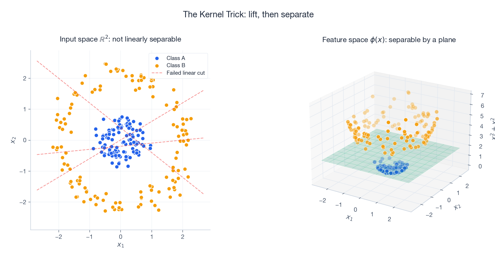
The kernel trick trades an explicit map $x \mapsto \phi(x)$ for an implicit one defined by a similarity function $K(x, y)$.
The picture above makes this concrete. In input space, the two classes form concentric rings: no straight line separates them. Lift each point with $\phi(x) = (x_1, x_2, x_1^2 + x_2^2)$ and the rings sit at different heights – now a flat plane separates them. The polynomial kernel $K(x, y) = (\langle x, y\rangle + 1)^2$ corresponds to all degree-2 polynomial features, but you compute one dot product instead of storing $O(d^2)$ extra coordinates.
Mathematical Foundation
Three results turn the kernel trick from a clever hack into a theory: positive-definite kernels (when is $K$ a valid inner product?), Mercer’s theorem (what does the implicit feature space look like?), and the RKHS construction (what function class are kernel methods optimising over?).
Positive-definite kernels
A symmetric function $K: \mathcal{X} \times \mathcal{X} \to \mathbb{R}$ is positive definite if for every finite set $\{x_1, \dots, x_n\}$ and every real vector $c \in \mathbb{R}^n$,
$$\sum_{i,j=1}^n c_i c_j \, K(x_i, x_j) \;\geq\; 0.$$Equivalently, the Gram matrix $K_{ij} = K(x_i, x_j)$ is positive semi-definite (PSD) for any sample of points.
Why this matters: positive-definite kernels are exactly the functions that arise as inner products in some Hilbert space. So picking a PD kernel is equivalent to picking an implicit feature map – you just don’t have to write it down.
Mercer’s theorem
If $K$ is continuous, symmetric, and positive definite on a compact set, then it has a spectral decomposition
$$K(x, y) \;=\; \sum_{k=1}^{\infty} \lambda_k \, \phi_k(x) \, \phi_k(y), \qquad \lambda_k \geq 0,$$where the $\phi_k$ are orthonormal eigenfunctions and the $\lambda_k$ are non-negative eigenvalues. The implicit feature map is
$$\phi(x) \;=\; \big(\sqrt{\lambda_1}\,\phi_1(x),\; \sqrt{\lambda_2}\,\phi_2(x),\; \dots\big).$$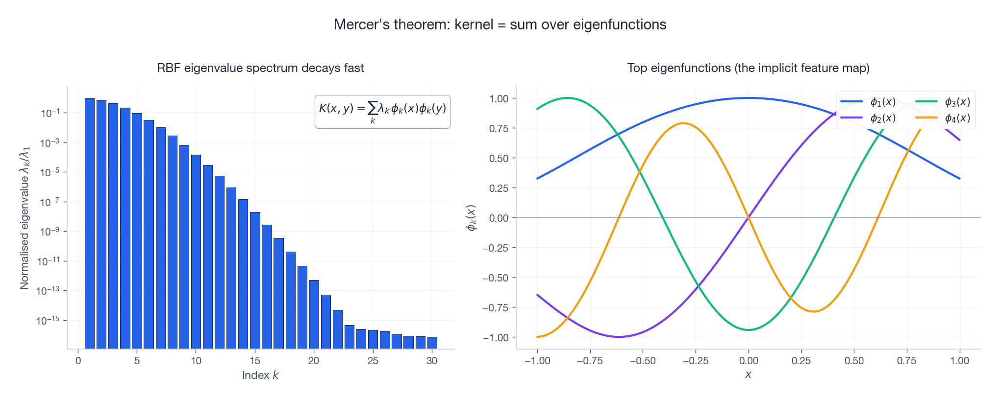
Two things to read off the figure:
- Eigenvalues decay fast. A handful of components carries almost all the kernel’s “mass”. This is why kernel methods admit good low-rank approximations (Nystrom, random Fourier features).
- Eigenfunctions look like Fourier modes. For the RBF kernel on an interval, the top eigenfunctions are smooth, increasingly oscillatory bumps – the kernel implicitly measures similarity in a smooth-function basis.
For the RBF kernel, the spectrum is infinite: every $\lambda_k > 0$. That is what people mean when they say “RBF has an infinite-dimensional feature space”.
Reproducing Kernel Hilbert Space (RKHS)
The Moore-Aronszajn theorem says: every positive-definite kernel uniquely defines a Hilbert space of functions $\mathcal{H}_K$ with two properties:
- Every $f \in \mathcal{H}_K$ is a function $\mathcal{X} \to \mathbb{R}$.
- Reproducing property. $f(x) = \langle f, K(x, \cdot) \rangle_{\mathcal{H}_K}$ for all $f \in \mathcal{H}_K$ and $x \in \mathcal{X}$.
The reproducing property is what makes RKHS theory powerful: function evaluation is a bounded linear operation, given by an inner product against $K(x, \cdot)$.
The practical consequence is the representer theorem. When you minimise a regularised risk
$$\min_{f \in \mathcal{H}_K} \;\frac{1}{n}\sum_i L(y_i, f(x_i)) \;+\; \lambda \|f\|_{\mathcal{H}_K}^2,$$the optimal $f^*$ always lies in the finite-dimensional subspace spanned by $\{K(x_i, \cdot)\}_{i=1}^n$:
$$f^*(x) \;=\; \sum_{i=1}^n \alpha_i \, K(x_i, x).$$You only ever need $n$ coefficients $\alpha_i$, no matter how infinite-dimensional $\mathcal{H}_K$ is. That is the structural reason kernel SVMs and Gaussian processes are tractable.
The Kernel Trick in Action
Kernel SVM
The dual of the soft-margin SVM is
$$\max_{\alpha} \;\sum_i \alpha_i \;-\; \tfrac{1}{2}\sum_{i,j} \alpha_i \alpha_j y_i y_j \,\langle x_i, x_j \rangle, \qquad 0 \leq \alpha_i \leq C.$$The data appears only through the inner product $\langle x_i, x_j\rangle$. Replace it with $K(x_i, x_j)$ and you have a non-linear classifier with the same optimisation problem, same number of variables, same solver. The decision function becomes
$$f(x) \;=\; \sum_{i \in \mathrm{SV}} \alpha_i y_i \, K(x_i, x) + b.$$Kernel PCA
Standard PCA eigendecomposes the $d \times d$ covariance matrix. Kernel PCA eigendecomposes the $n \times n$ centred Gram matrix instead. The top eigenvectors $\alpha^{(k)}$ give projections
$$z_k(x) \;=\; \sum_{i=1}^n \alpha_i^{(k)} \, K(x_i, x),$$which extract non-linear principal components without ever materialising $\phi(x)$.
Kernel ridge regression
The minimiser of $\sum_i (y_i - f(x_i))^2 + \lambda \|f\|^2_{\mathcal{H}_K}$ has a closed form,
$$\hat{f}(x) = \mathbf{k}(x)^\top (K + \lambda I)^{-1} \mathbf{y},$$where $\mathbf{k}(x)_i = K(x_i, x)$. This is also the posterior mean of a Gaussian process with covariance $K$ and noise $\lambda$.
Common Kernels: Theory and Practice
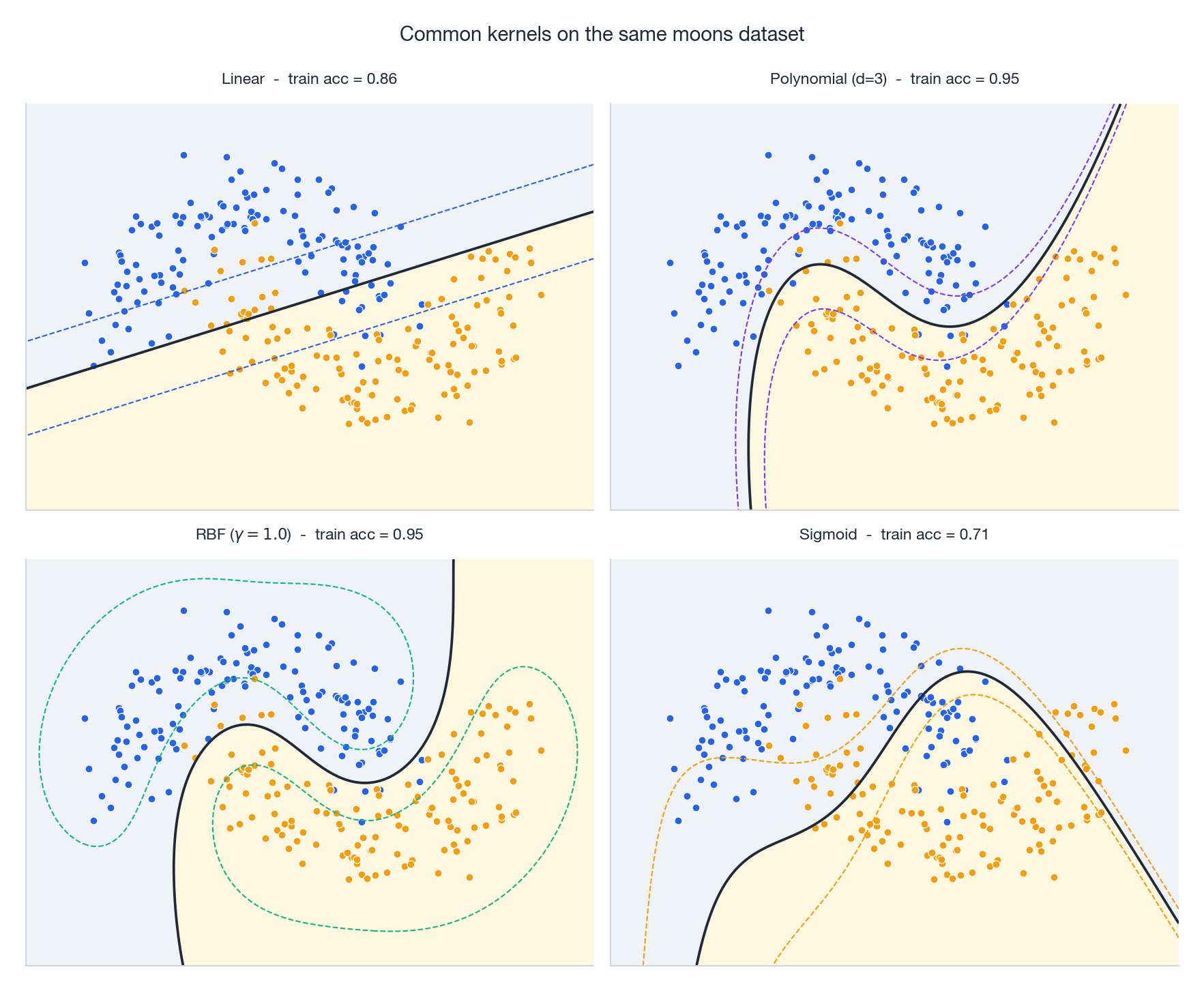
Pick one dataset, swap the kernel, and the decision boundary changes character entirely. Linear can’t bend, polynomial bends in algebraic shapes, RBF wraps tightly around the data, sigmoid often misbehaves. Below is the working manual.
1. RBF (Gaussian) kernel
$$K(x, y) = \exp\!\left(-\gamma \,\|x - y\|^2\right) \quad \text{or} \quad \exp\!\left(-\frac{\|x-y\|^2}{2\sigma^2}\right).$$(scikit-learn uses $\gamma$; many textbooks use $\sigma$. The relation is $\gamma = 1/(2\sigma^2)$.)
Properties. Infinite-dimensional feature space, infinitely differentiable, universal (it can approximate any continuous function on a compact set, given enough data and the right bandwidth).
When to use. The default for SVM, GP, and kernel PCA. Good whenever you expect smooth, local structure.
Hyperparameter $\gamma$ (or $\sigma$). This single number controls the influence radius and is by far the most consequential choice you make.
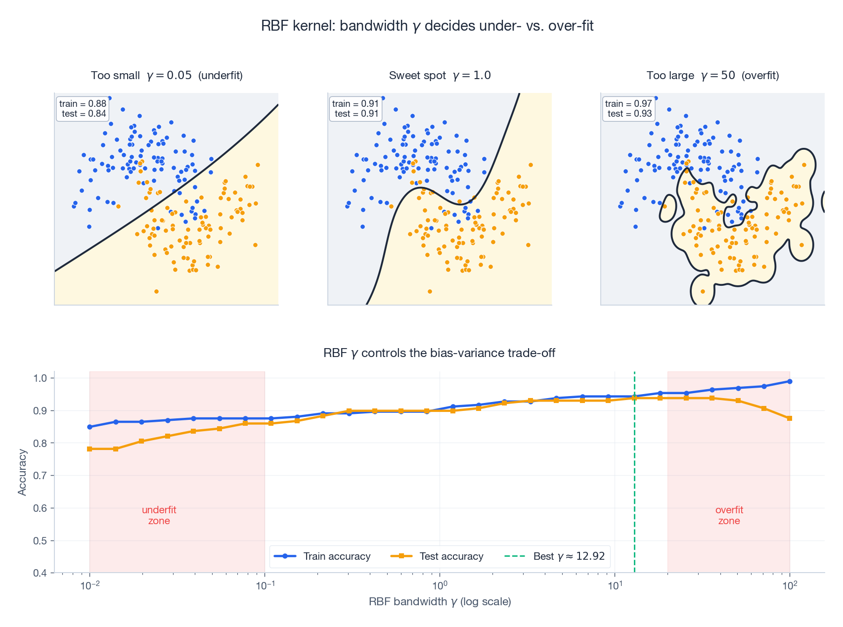
- $\gamma$ too large (small $\sigma$): each training point only influences itself. The Gram matrix becomes nearly the identity; the model memorises the training set; test accuracy collapses.
- $\gamma$ too small (large $\sigma$): every point looks the same to every other point; the kernel acts like a constant; the model underfits.
- Sweet spot. Found by cross-validation on a log grid. A reasonable starting point is the median heuristic: $\sigma \approx \mathrm{median}(\|x_i - x_j\|)$, equivalently $\gamma \approx 1/(2 \cdot \mathrm{median}^2)$.
2. Polynomial kernel
$$K(x, y) = (\gamma\, \langle x, y \rangle + c)^d.$$Properties. Finite-dimensional feature space (all monomials up to degree $d$). Captures explicit interactions of order up to $d$.
When to use. Sparse high-dimensional data with known interactions (text classification with bigrams; genomics with epistasis). Avoid for dense low-dimensional data – RBF usually wins.
Hyperparameters. $d \in \{2, 3\}$ in practice; degree-$5+$ polynomials almost always overfit. $\gamma$ scales the inner product (sensitive to feature magnitudes; normalise first). $c$ controls the trade-off between low- and high-order terms; $c = 0$ keeps only top-order monomials, $c = 1$ mixes all orders.
3. Linear kernel
$$K(x, y) = \langle x, y \rangle.$$The trivial kernel. No feature mapping, $O(d)$ per evaluation, equivalent to running the linear algorithm directly.
When to use. Linearly separable data, very high-dimensional sparse data (text, gene expression), or as a baseline. For text in particular, linear SVMs often beat RBF – the curse of dimensionality is on your side here, since random points in high-$d$ space are nearly orthogonal.
4. Sigmoid kernel
$$K(x, y) = \tanh(\gamma\, \langle x, y \rangle + c).$$Modelled after a neural network activation, but not always positive definite – only for certain ranges of $\gamma, c$. Modern practice has largely abandoned it: if you want neural-network-style nonlinearity, train a neural network. Keeping it here mostly so you recognise it in legacy code.
5. Matern kernel (Gaussian processes)
$$K_\nu(r) = \frac{2^{1-\nu}}{\Gamma(\nu)} \left(\frac{\sqrt{2\nu}\, r}{\ell}\right)^{\!\nu} \! K_\nu\!\left(\frac{\sqrt{2\nu}\, r}{\ell}\right), \qquad r = \|x - y\|.$$The Matern kernel has a tunable smoothness parameter $\nu$:
- $\nu = 1/2$: exponential kernel; sample paths are continuous but nowhere differentiable. Good for rough functions.
- $\nu = 3/2$: sample paths are once differentiable.
- $\nu = 5/2$: twice differentiable. The most common choice in Bayesian optimisation.
- $\nu \to \infty$: recovers RBF (infinitely smooth).
When to use. Almost always preferable to RBF for Gaussian-process regression. RBF’s infinite smoothness is unrealistically strong for most real functions; Matern with $\nu = 5/2$ is the workhorse default.
6. Periodic kernel (time series)
$$K(x, y) = \exp\!\left(-\frac{2 \sin^2(\pi \|x - y\| / p)}{\ell^2}\right).$$Captures strict periodicity with period $p$. Combine additively with an RBF or linear kernel to model “trend + seasonality”.
When to use. Time series with seasonality (temperature, electricity load, sales). Audio pitch tracking. Any signal with a known periodic component.
Hyperparameter Tuning
Cross-validation (the default)
Split the data into $k$ folds, train on $k-1$, validate on the held-out fold, average. Pick the hyperparameter combination with the best average validation score.
| |
For higher-dimensional hyperparameter spaces, random search is more sample-efficient than grid search:
| |
Marginal likelihood (Gaussian processes)
For GP regression you can tune $\theta$ (the kernel hyperparameters) by maximising the log marginal likelihood
$$\log p(\mathbf{y} \mid \theta) = -\tfrac{1}{2} \mathbf{y}^\top (K_\theta + \sigma^2 I)^{-1} \mathbf{y} \;-\; \tfrac{1}{2} \log |K_\theta + \sigma^2 I| \;-\; \tfrac{n}{2}\log(2\pi).$$This is principled (no held-out set needed) and decomposes into a fit term, a complexity penalty, and a constant – Occam’s razor falls out of the math. Caveat: with noisy data and many hyperparameters, marginal-likelihood optimisation can overfit; add weak priors (e.g., log-normal) on length scales.
Diagnostics: Read the Gram Matrix
The kernel matrix itself tells you whether your hyperparameters are sane.
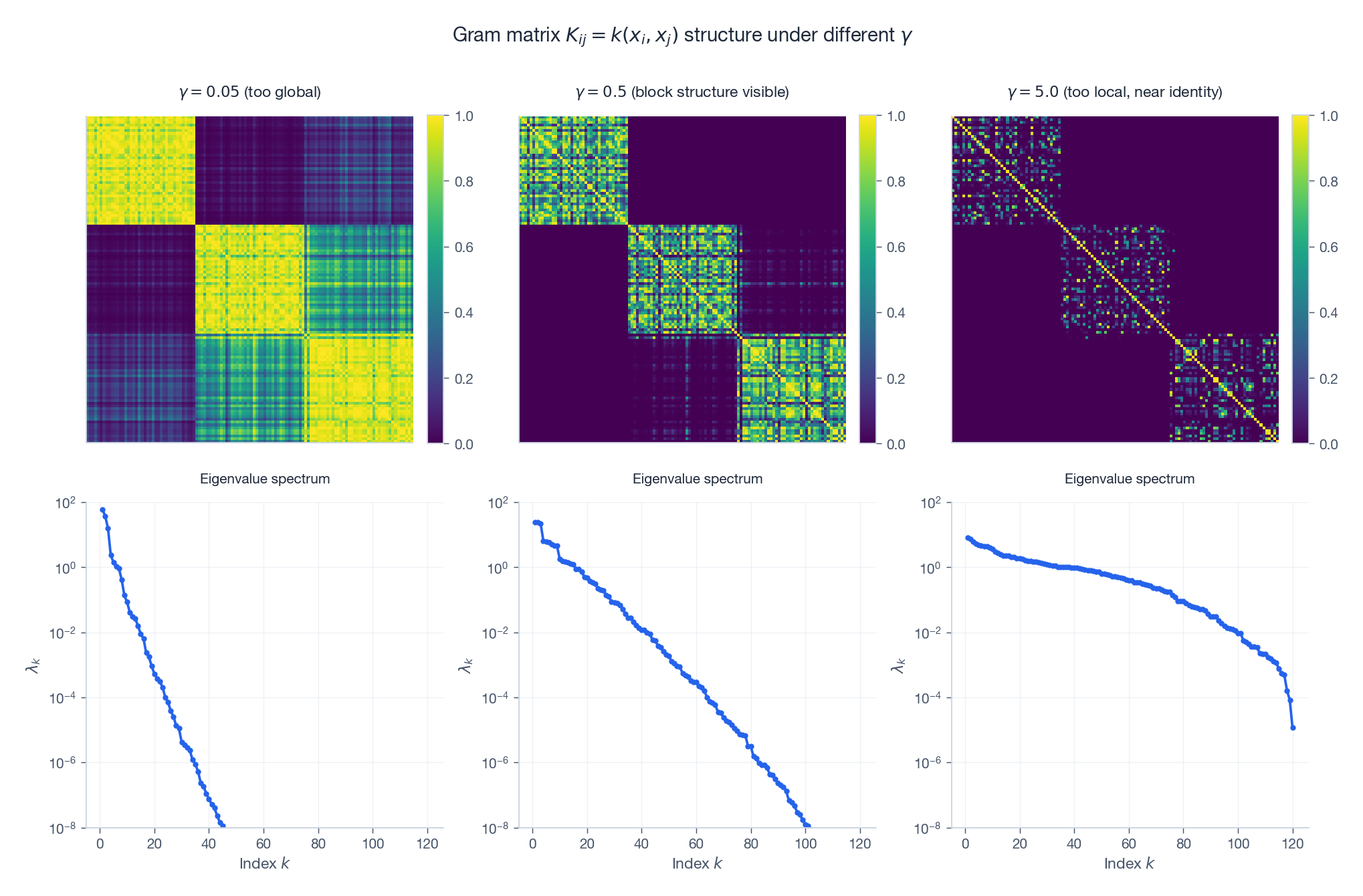
Three regimes for an RBF kernel on three Gaussian clusters (rows sorted by cluster):
- $\gamma$ too small. The matrix is uniformly bright – every pair of points looks similar. The eigenvalue spectrum is dominated by one mode. Underfit.
- $\gamma$ in the sweet spot. Three crisp diagonal blocks emerge, one per cluster. The spectrum has a clear three-step staircase. The kernel sees the cluster structure.
- $\gamma$ too large. The matrix collapses to the identity. The spectrum is flat. Every point is its own island; no generalisation possible.
A two-line check during development:
| |
Troubleshooting Guide
Problem 1: overfitting
Symptoms. Training accuracy near 1.0; test accuracy much lower; Gram matrix looks near-diagonal.
Causes. RBF $\gamma$ too large (small bandwidth), polynomial degree too high, SVM $C$ too large (insufficient regularisation).
Fixes. Decrease $\gamma$. Lower polynomial degree. Decrease $C$. Increase GP noise variance. Get more training data.
Problem 2: underfitting
Symptoms. Training and test accuracy both poor. Predictions almost constant.
Causes. Linear kernel on non-linear data. RBF $\gamma$ too small. SVM $C$ too small.
Fixes. Move up the expressiveness ladder: linear $\to$ polynomial $\to$ RBF. Increase $\gamma$. Increase $C$.
Problem 3: numerical instability
Symptoms. GP fit fails with “singular matrix”; kernel-PCA returns negative eigenvalues; SVM solver does not converge.
Causes. The Gram matrix is rank-deficient or ill-conditioned. Often caused by duplicate points, an invalid (non-PSD) custom kernel, or extremely small $\gamma$.
Fixes.
- Add jitter to the diagonal:
K = K + 1e-6 * np.eye(n). - Standardise features before RBF/Matern – distance-based kernels are scale-sensitive.
- Drop near-duplicate rows.
- Use a 64-bit dtype for the kernel matrix.
- Verify PSD for custom kernels:
np.all(np.linalg.eigvalsh(K) >= -1e-8).
Problem 4: training is too slow
Symptoms. SVM takes hours on $10^4$ samples; GP regression infeasible past a few thousand.
Cause. Kernel methods are $O(n^2)$ memory and $O(n^3)$ compute (matrix factorisation).
Fixes.
- Linear kernel if it suffices: scales to millions with
LinearSVC/ SGD. - Nystrom approximation (
sklearn.kernel_approximation.Nystroem): pick $m \ll n$ landmarks, get an explicit $m$-dim feature map. - Random Fourier features for translation-invariant kernels (RBF, Matern): explicit map of dimension $D$, error decays as $1/\sqrt{D}$.
- Sparse / inducing-point GPs (
gpytorch,GPy): scale GPs to $10^5$ samples. - Switch to deep learning when $n \gtrsim 10^5$ and structure is complex.
Kernel Selection Decision Tree
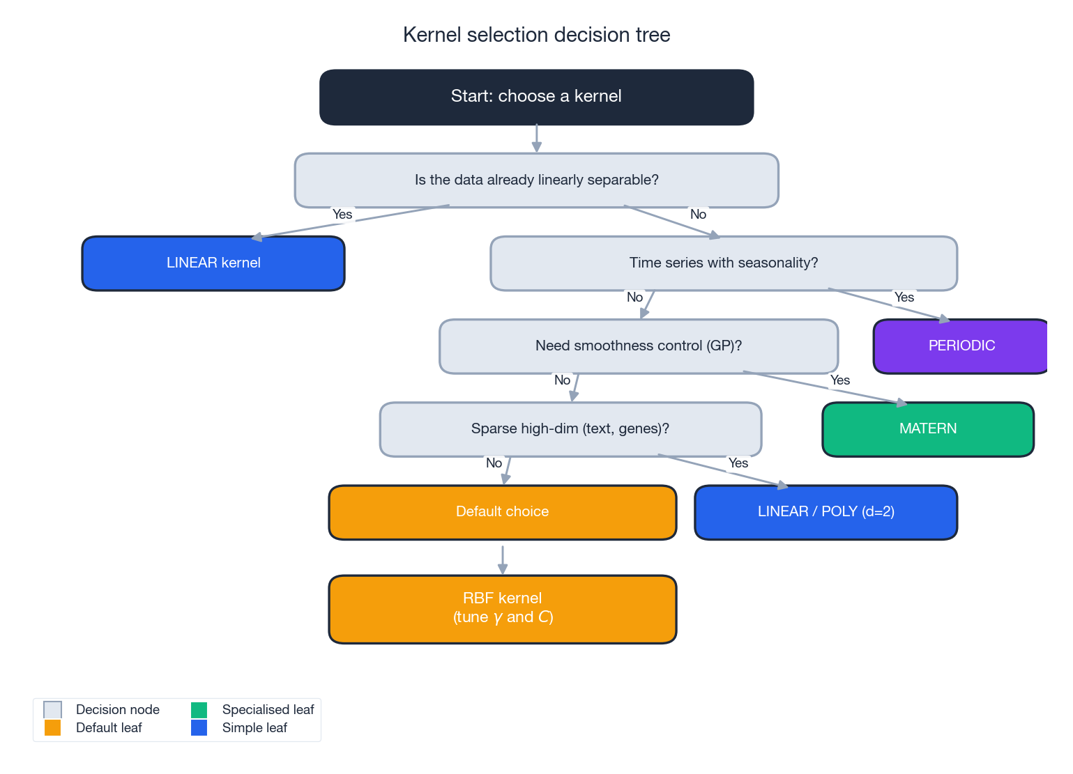
The flow:
- Linearly separable already? Use the linear kernel. Fast, interpretable, hard to beat for sparse high-dim data.
- Time series with strong seasonality? Use a periodic kernel (often added to a smooth kernel).
- Need fine-grained control over function smoothness (typically GPs)? Use a Matern kernel; pick $\nu$ from $\{1/2, 3/2, 5/2\}$.
- Sparse, high-dim data with known interactions (text, genomics)? Try linear first, then polynomial with $d = 2$.
- Otherwise. Default to RBF and tune $\gamma$ and $C$ on a log grid.
Practical Tips
1. Always standardise features. RBF and Matern are distance-based; a feature measured in millions will dominate one measured in fractions. StandardScaler (or RobustScaler for heavy-tailed features) before the kernel, every time.
2. Search on a log scale. Hyperparameters like $\gamma$, $C$, and $\sigma$ act multiplicatively. A linear grid spends most of its budget in a narrow band; a log grid covers many orders of magnitude with the same number of points.
3. Build the model in a Pipeline. Pipeline([scaler, kernel_model]) ensures the scaler is fit on each CV training fold, not on the whole dataset – otherwise you leak test statistics into validation.
4. Compose kernels. Sums and products of valid kernels are valid kernels. Matern * Periodic + WhiteNoise is a standard recipe for “smooth, seasonal, with noise”.
5. Sanity-check custom kernels.
| |
Kernel Methods vs. Deep Learning
| Aspect | Kernel methods | Deep learning |
|---|---|---|
| Training data | Excellent with small data ($n < 10^4$) | Needs large data ($n \gtrsim 10^5$) |
| Interpretability | High (RKHS, support vectors) | Low (largely black-box) |
| Hyperparameters | Few (kernel params + regularisation) | Many (architecture, optimiser, schedule, …) |
| Scaling | Poor ($O(n^2)$ memory, $O(n^3)$ compute) | Good (mini-batch, GPU) |
| Theory | Strong (RKHS, Mercer, representer theorem) | Mostly empirical |
| Uncertainty | Native via Gaussian processes | Add-on (ensembles, MC dropout, BNN) |
Use kernel methods when you have small to mid-size data, want calibrated uncertainty (GPs), or value interpretability (SVM support vectors).
Use deep learning when you have large data, need to learn representations from raw signals (images, audio, text), or care about scaling.
These choices are not mutually exclusive. Deep kernel learning uses a neural network as a learned feature extractor and a Gaussian process on top – the best of both worlds when applicable.
Summary: Kernel Methods in Five Steps
- Pick the family. Linearly separable $\to$ linear. Otherwise default to RBF; use Matern for GPs, periodic for seasonal time series.
- Standardise features. Non-negotiable for RBF / Matern / periodic.
- Tune on a log grid. Cross-validate $\gamma$, $C$, polynomial degree, length scale.
- Read the diagnostics. Plot the Gram matrix; near-diagonal $\to$ overfit (decrease $\gamma$); near-uniform $\to$ underfit (increase $\gamma$).
- Scale up if needed. Linear kernel for $n \to 10^6$; Nystrom / random features for non-linear; sparse GPs for probabilistic models; deep learning when structure dominates.
Key hyperparameters at a glance.
- RBF. $\gamma$ (bandwidth), $C$ (regularisation).
- Polynomial. $d$ (degree, keep $\leq 3$), $\gamma$, $c$.
- Matern. $\nu$ (smoothness, fix to $5/2$ unless you know better), $\ell$ (length scale).
Common pitfalls.
- Forgetting to standardise features (RBF fails silently with worse-than-random accuracy).
- Using the sigmoid kernel (often non-PSD; pick something else).
- Searching $\gamma$, $C$ on a linear grid (you waste 90 % of the search budget).
- Fitting the scaler on the full dataset before CV (leaks test info into training).
Further Reading
- Hofmann, Scholkopf, Smola. Kernel Methods in Machine Learning (Annals of Statistics, 2008). The canonical survey.
- Rasmussen and Williams. Gaussian Processes for Machine Learning (MIT Press, 2006). Free PDF; the GP bible.
- Scholkopf and Smola. Learning with Kernels (MIT Press, 2002). The textbook treatment.
- Rahimi and Recht. Random Features for Large-Scale Kernel Machines (NeurIPS, 2007). The random Fourier features paper.
- Wilson and Adams. Gaussian Process Kernels for Pattern Discovery and Extrapolation (ICML, 2013). Spectral mixture kernels for time series.