Your model diverges. You halve the learning rate. Now it trains, but takes forever. You halve again — now the loss is a flat line. Sound familiar? Of all the knobs you can turn, learning rate is the one that most often decides whether training converges, crawls, or blows up. This guide gives you the intuition, the minimal math, and a practical workflow to get it right — from a 12-layer CNN on your laptop to a 70B-parameter LLM on a thousand GPUs.

What you will learn

• Why “too big explodes, too small stalls” — derived from the simplest possible model
• How batch size, momentum, and weight decay couple with LR (you cannot tune one in isolation)
• The schedule zoo — constant, step, cosine, WSD, schedule-free — and when to use which
• The LR range test: how to find your stability boundary in 200 mini-batches
• A diagnostic checklist for NaN losses, plateaus, and oscillations
• What’s new since 2023 — Schedule-Free AdamW, D-Adaptation, Power Scheduler, the new theory of warmup

Prerequisites: basic calculus (gradients, chain rule) and you have trained at least one neural network.

1. The one-sentence definition

Learning rate $\eta$ controls how far you move along the direction the gradient suggests, each step.

The basic update rule is

where $\tilde g_t$ is usually a mini-batch (stochastic) estimate of the true gradient $\nabla L(\theta_t)$.

The core trade-off:

$\eta$ large → fast progress, but unstable. $\eta$ small → stable, but slow (or stuck).

The rest of this article is, essentially, the story of how researchers and engineers have learned to walk this tightrope.

2. Why “too big explodes, too small stalls”

2.1 A 1-D quadratic — the cleanest possible intuition

Take the simplest non-trivial loss:

The gradient is $\nabla L(\theta) = a\theta$, so gradient descent gives

The whole trajectory is now a geometric sequence with ratio $r = 1 - \eta a$. Three regimes pop out:

• $|r| < 1 \Leftrightarrow 0 < \eta < 2/a$ — converges to 0.
• $|r| = 1 \Leftrightarrow \eta = 2/a$ — bounces forever.
• $|r| > 1 \Leftrightarrow \eta > 2/a$ — blows up.

So the stability ceiling is $\eta < 2/a$, where $a$ is the curvature. Bigger curvature → smaller maximum stable LR. The picture below shows all three regimes on the same loss bowl.

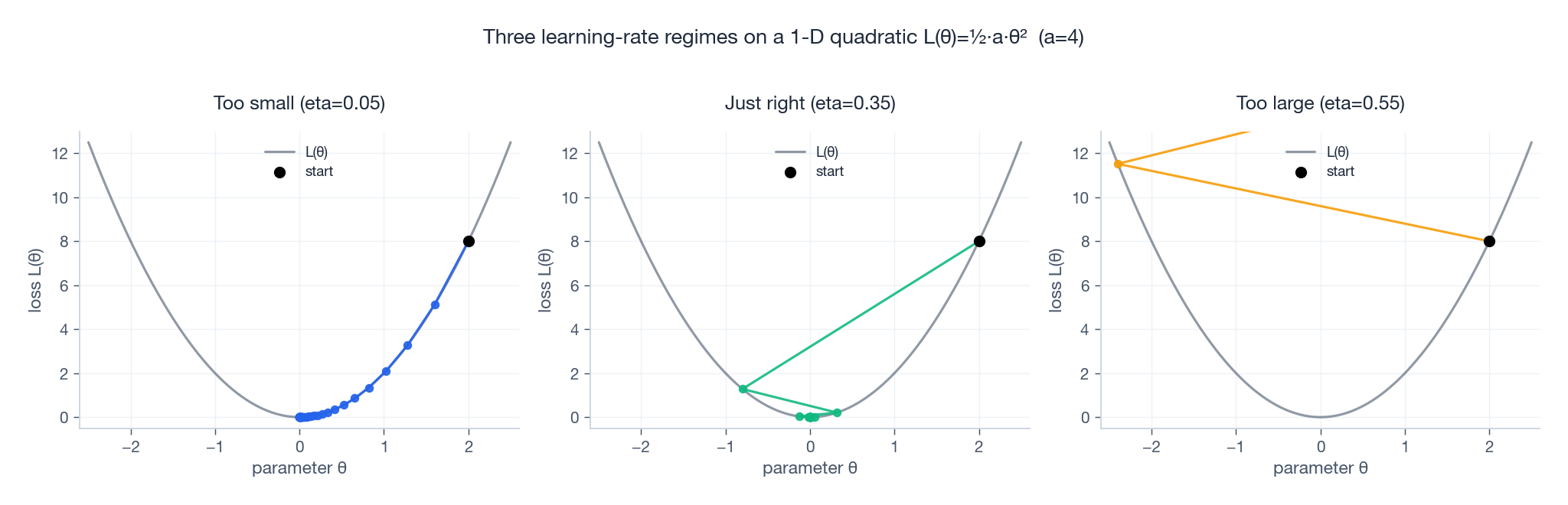
Notice in the right panel that the iterate doesn’t just overshoot — it bounces with growing amplitude. That’s the geometric explosion that turns into NaN in real training.

2.2 In high dimensions: the steepest direction sets the ceiling

Real losses are not 1-D quadratics, but locally a quadratic approximation $L(\theta) \approx \tfrac{1}{2} (\theta - \theta^\star)^\top H (\theta - \theta^\star)$ is a fine model. The Hessian $H$ has eigenvalues $\lambda_1 \geq \dots \geq \lambda_n \geq 0$, and stability now requires

Key insight: it does not matter how gentle most directions are — a single sharp direction (the largest eigenvalue) sets the ceiling for the entire optimizer. You’re walking a wide valley, but one cliff edge is enough to make you fall.

This is also why training feels harder than it “should”: the largest eigenvalue grows during training (this phenomenon is called progressive sharpening, see Cohen et al. 2021), so the LR you got away with at step 100 may blow up at step 10 000.

2.3 $L$-smoothness: where the textbook bound $\eta \leq 1/L$ comes from

Generalize beyond quadratics. A function is $L$-smooth if its gradient is $L$-Lipschitz:

Intuitively: the loss surface has no “infinitely sharp” direction; curvature is bounded by $L$. Under this assumption, classical analysis shows that gradient descent with $\eta \leq 1/L$ never increases the loss. The exact form is the descent lemma

which is monotonically decreasing for $\eta < 2/L$ and most aggressively decreasing at $\eta = 1/L$. This is the “safe choice” — it’s also why $L$ and the maximum eigenvalue $\lambda_{\max}(H)$ play essentially the same role.

2.4 Why schedules exist at all

In real networks the curvature, the gradient noise, and even the eigenvector directions all change as training progresses. No constant LR is right for the whole run. A typical schedule does three things in sequence:

• Warmup — the curvature is huge and parameters are random; ramp $\eta$ up slowly.
• Stable / high LR — curvature has settled; harvest fast progress.
• Decay / cooldown — averaged gradient is small but noise is constant; shrink $\eta$ to settle into the basin.

The best way to picture this is to plot the standard schedules on one chart.

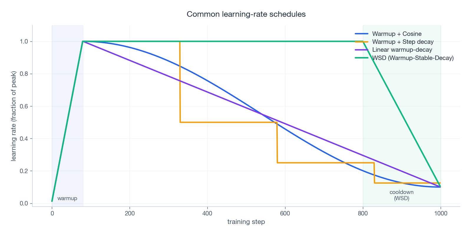
We will dissect each of these in §5.

3. Batch size, momentum, weight decay: the hidden coupling

You cannot tune LR in isolation. Three friends always travel with it.

3.1 Batch size and the linear scaling rule

The mini-batch gradient $\tilde g_t$ is an unbiased estimate of $\nabla L(\theta_t)$ with variance roughly $\sigma^2 / B$, where $B$ is the batch size. So:

• larger batch → less noise → larger LR is safe.
• smaller batch → more noise → larger LR causes random “kicks” that diverge.

The classical empirical rule (Goyal et al. 2017, “Accurate, Large Minibatch SGD”) is the linear scaling rule: if you increase $B$ by $k$, multiply $\eta$ by $k$. But add warmup — early training is so unstable that the linear rule alone overshoots.

Modern large-batch results (LAMB, LARS) extend this idea, but the basic message is unchanged: LR and $B$ are tied.

3.2 Momentum: a hidden LR amplifier

SGD with momentum (Polyak / heavy-ball form):

In steady state, $v_t \approx g / (1 - \beta)$, so the effective step size is roughly $\eta / (1 - \beta)$. With the typical $\beta = 0.9$, momentum multiplies your effective LR by 10×. That’s why SGD-with-momentum recipes often use a smaller $\eta$ than what bare SGD could tolerate — the momentum is doing half the gas-pedal work.

Adam’s first moment is similar in spirit.

3.3 Weight decay: a coupled regularizer

Decoupled weight decay (AdamW) is

so the “shrinkage” applied per step is $\eta \lambda$. Doubling LR also doubles your effective weight decay. The steady-state weight norm is roughly $\propto \sqrt{1/\lambda}$, independent of $\eta$, but how fast you reach it depends on $\eta$. This is why “lower $\eta$ → less regularization” is a real and frequently-overlooked effect.

Practical rule: when retuning LR, retune weight decay in the same sweep.

4. Adaptive optimizers: per-parameter learning rates

If SGD’s LR is one big hammer, Adam is a workshop full of small hammers — each parameter gets its own.

4.1 The Adam update

The key term is $\eta / \sqrt{\hat v_t}$ — the effective per-parameter LR scales like $\eta / |g|$. Parameters with consistently large gradients get small steps; quiet parameters get full $\eta$. That is why Adam works out-of-the-box on dramatically different scales (embeddings, attention, layer norms) where SGD would need careful per-layer LR.

4.2 Why Adam still needs warmup

It’s tempting to think the adaptive scaling makes warmup unnecessary. It doesn’t. Two reasons:

• Statistics are unstable early. $\hat v_t$ is computed from a few noisy gradients; the bias correction divides by $(1 - \beta_2^t)$, which is huge for small $t$. This used to be the textbook explanation.
• Preconditioned sharpness is large. The newer view (Kalra et al., Why Warmup the Learning Rate?, 2024) is that warmup pushes the network into a region where the preconditioned Hessian has smaller maximum eigenvalue — i.e. it shapes the optimization landscape, so a larger peak LR becomes safe later.

Either way: always warm up Adam. 1–5% of total steps for vision/CNN, 5–10% for LLMs and very large batches.

5. Schedules: from old-school to modern LLMs

The plot above shows four common families on one axis. Here is when to reach for which.

5.1 Constant LR

Simple. Almost always wrong. Either too slow early or too noisy late — you cannot have both.

5.2 Step decay

Multiply $\eta$ by $\gamma$ (typically 0.1) at fixed milestones. The classic ResNet recipe. Pros: easy to implement, easy to tune by hand. Cons: the abrupt drop can cause loss spikes if your weight decay or batch normalization is sensitive.

5.3 Cosine decay (the deep-learning workhorse)

after a linear warmup of length $t_w$. The shape — slow decay early, fast decay late — matches the intuition: explore at high $\eta$ for as long as possible, then settle.

This was the schedule of choice for almost every “big model” paper between 2019 and 2023 (BERT, RoBERTa, GPT-3, ViT, ResNet on ImageNet at scale). Its main drawback is rigidity: the cosine half-period is set by the known total step count $T$. If you want to extend the run, you have to redesign the schedule.

5.4 WSD: warmup–stable–decay (the modern LLM default)

Hägele et al. (Scaling Laws and Compute-Optimal Training Beyond Fixed Training Durations, 2024) and others have popularized WSD:

• Warmup — same as before.
• Stable — hold $\eta = \eta_{\max}$ for the bulk of training (60–90%).
• Cooldown — linearly (or polynomially) drop to $\eta_{\min}$ in the last 10–20%.

Three reasons it has become the LLM default:

1. Resumable / extensible. Want 2× more tokens? Just continue the stable phase, then cooldown later. Cosine cannot do this without re-fitting the full curve.
2. The “cooldown drop” effect. Empirically, when cooldown starts the loss often takes a sharp final dip — as if the model had been “barely held back” and was finally allowed to settle.
3. Theoretical backing. Schaipp et al. (The surprising agreement between convex optimization theory and learning-rate scheduling, 2025, arXiv:2501.18965) showed that the cooldown shape matches a tight bound from convex theory, with cooldown specifically removing log-factor terms.

5.5 Cosine vs WSD vs Schedule-Free at a glance

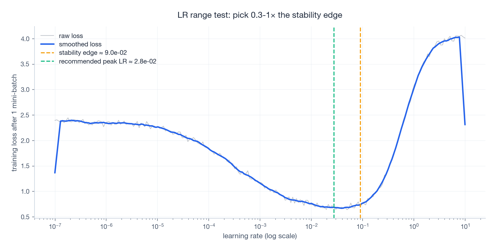
6. The LR range test: find your ceiling in 200 batches

The single most useful tool for picking $\eta_{\max}$, due originally to Smith (2015, Cyclical Learning Rates):

1. Set $\eta = \eta_{\min} \approx 10^{-7}$.
2. After every mini-batch, multiply $\eta$ by a fixed factor (e.g. 1.1) so it grows exponentially.
3. Stop when the loss starts climbing.
4. Plot loss against $\log\eta$.

You’ll see four phases: noisy plateau → descent → noisy minimum → blow-up. The “edge” is just before the blow-up; pick your peak LR somewhere in $[0.3 \times, 1.0 \times]$ that edge.

 1
 2
 3
 4
 5
 6
 7
 8
 9
10
11
12
13
14
15
16
17
18
19
20
21
22
23
24
25
26
27
28
29
30
31
32

import math
import torch

def lr_range_test(model, loader, loss_fn, optimizer,
                  lr_min=1e-7, lr_max=10, num_steps=200):
    """Run an exponential LR sweep; return (lrs, losses) for plotting."""
    model.train()
    mult = (lr_max / lr_min) ** (1 / (num_steps - 1))
    lr = lr_min
    for g in optimizer.param_groups:
        g["lr"] = lr

    lrs, losses = [], []
    it = iter(loader)
    for _ in range(num_steps):
        try:
            x, y = next(it)
        except StopIteration:
            it = iter(loader)
            x, y = next(it)

        optimizer.zero_grad(set_to_none=True)
        loss = loss_fn(model(x), y)
        loss.backward()
        optimizer.step()

        lrs.append(lr)
        losses.append(loss.item())
        lr *= mult
        for g in optimizer.param_groups:
            g["lr"] = lr
    return lrs, losses

A tidy variant smooths the loss with an exponential moving average and stops automatically once loss rises by more than $4\times$ the running minimum — that’s how fastai’s lr_find() is implemented.

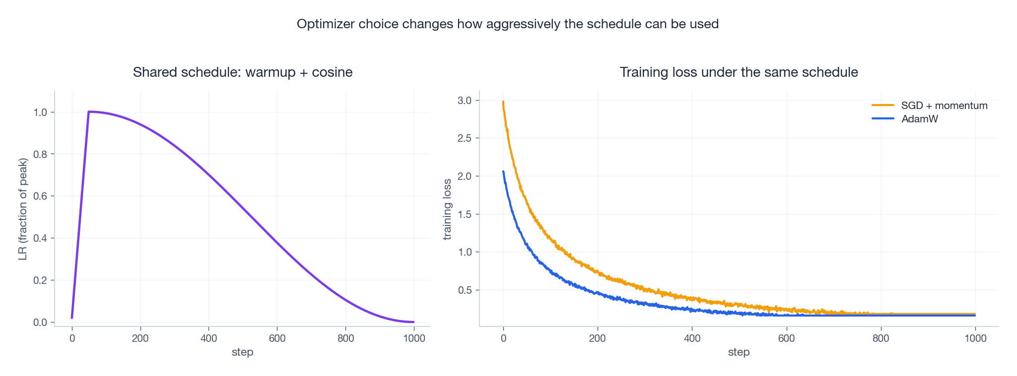
7. Optimizer choice changes the picture

The same schedule does not give the same loss curve under different optimizers. The figure below shares one warmup-cosine schedule between AdamW and SGD-with-momentum on a synthetic problem. AdamW descends faster early; SGD often catches up later but is more sensitive to the peak LR.

Practical heuristics, condensed from a decade of recipes:

• AdamW with lr ≈ 1e-4 ~ 5e-4 for Transformers and most NLP/multimodal pretraining.
• AdamW with lr ≈ 1e-5 ~ 5e-5 for fine-tuning pretrained Transformers.
• SGD + momentum 0.9 with lr ≈ 0.1 for ResNet/CNN training from scratch, with cosine or step decay.
• SGD + momentum when you want lower memory (no second-moment buffer) and have time to tune.

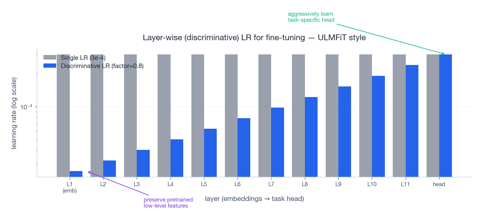
8. Layer-wise / discriminative LR: the fine-tuning trick

When you fine-tune a pretrained model, the lower layers already know how to extract good features — you don’t want to wash them away. The higher layers are random / task-specific and need much larger updates. This was popularized by ULMFiT (Howard & Ruder, 2018) as discriminative learning rates: use a small base LR for the top, and divide by a factor (e.g. 2.6 or 0.8 per group) as you go down.

A minimal PyTorch pattern:

 1
 2
 3
 4
 5
 6
 7
 8
 9
10

def layer_wise_param_groups(model, base_lr=3e-4, decay=0.8):
    """Assign smaller LR to layers closer to the input."""
    layers = list(model.encoder.layer)            # Hugging Face style
    groups = []
    n = len(layers)
    for i, layer in enumerate(layers):
        groups.append({"params": layer.parameters(),
                       "lr": base_lr * (decay ** (n - 1 - i))})
    groups.append({"params": model.classifier.parameters(), "lr": base_lr})
    return groups

For LLM fine-tuning the same idea reappears as:

• LoRA / adapters — train only a tiny set of new params at full LR; keep the rest frozen.
• LLaMA-Adapter style — gradually unfreeze, with a smaller LR for the unfrozen base.

9. Schedule-free and learning-rate-free optimizers

Both schedules and the LR scalar itself can, in principle, be eliminated. Two recent lines of work try to.

9.1 D-Adaptation (Defazio & Mishchenko, 2023)

D-Adaptation estimates the distance from initialization to optimum during training, and uses that estimate to set the step size. There is no $\eta$ to tune. On many tasks it matches a tuned baseline within a few percent.

9.2 Schedule-Free AdamW (Defazio et al., 2024, arXiv:2405.15682)

Schedule-Free AdamW combines iterate averaging with a constant base LR to produce trajectories that behave like cosine-decayed runs without ever explicitly decaying $\eta$. This means you don’t have to commit to a total step count $T$ upfront: you can stop whenever you like, or extend, without re-tuning.

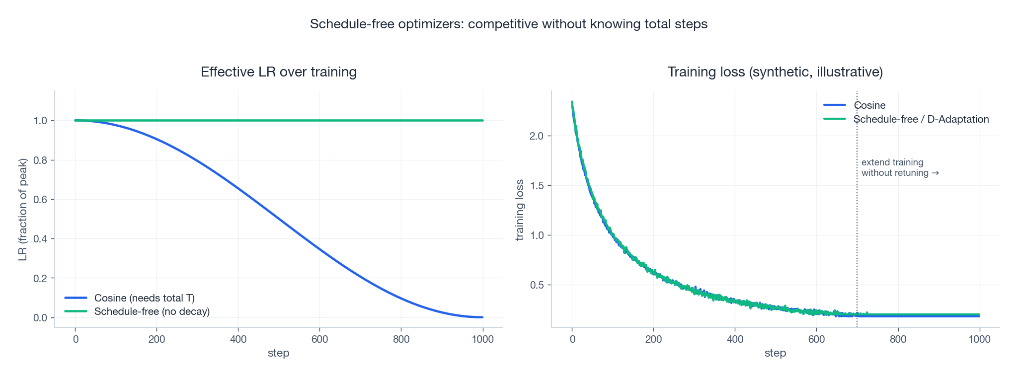
When to consider these:

• Prototyping; you don’t yet know your budget.
• Multi-budget studies (5%, 25%, 100% of tokens) where redoing cosine for each is painful.
• Compute-elastic settings (cluster preemption, reschedules).

10. What an LLM schedule actually looks like

The schedule used by GPT-3 (175B) and LLaMA (7B/13B/65B) is the same template: linear warmup over a small fraction of steps, then cosine decay to 10% of the peak LR. The peak itself depends on model size (bigger model → smaller peak, roughly $\eta_{\max} \propto 1/\sqrt{N}$ in the GPT scaling laws).

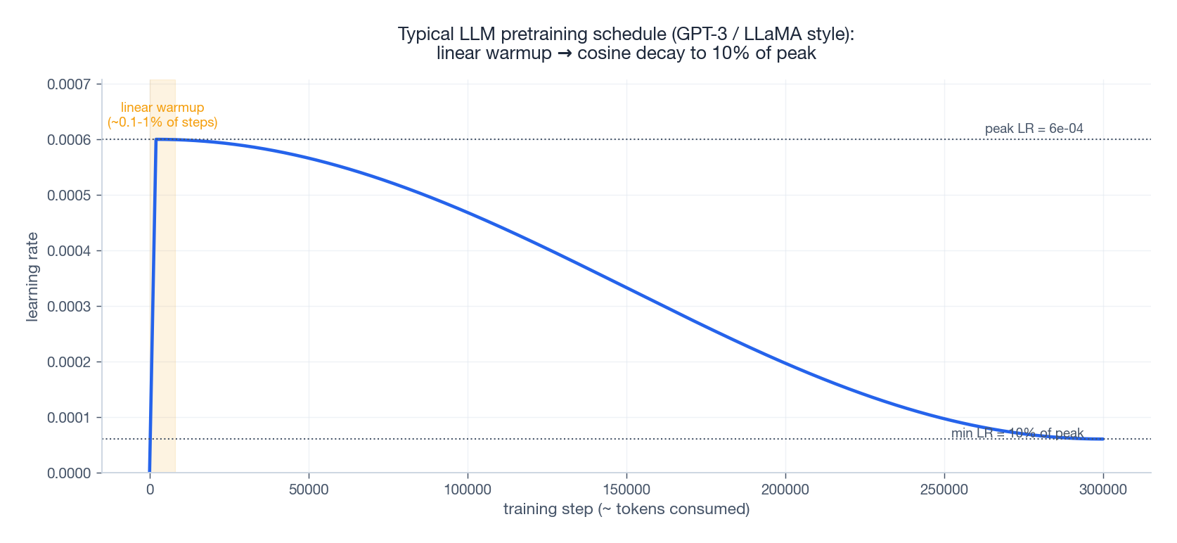
Concrete numbers from public papers:

A few things worth noting:

• Min LR ≈ 10% of peak LR is the near-universal convention, not zero. Going to zero often makes the very last steps useless.
• Gradient clipping at 1.0 is universal in this regime; without it, the occasional bad batch can knock you off the cliff.
• Weight decay 0.1 (decoupled, AdamW) is another common default in LLM recipes — much higher than the 1e-4 you see in vision.

11. From “it runs” to “it works”: a practical workflow

Step 1 — diagnose the failure mode

Training fails in three distinct flavours:

Step 2 — find your ceiling

Run an LR range test (§6). Most “I tried 1e-3 and 1e-4, both bad” stories are solved here.

Step 3 — choose the schedule

Step 4 — co-tune LR with batch and weight decay

Don’t change LR in isolation. The mental model is a three-way coupling:

Step 5 — monitor three things, not just loss

• Gradient norm. Should be roughly constant after warmup; sudden spikes precede divergence.
• Update / parameter ratio. $\|\Delta\theta\| / \|\theta\|$ around $10^{-3}$ is healthy. Below $10^{-5}$ → underfit; above $10^{-2}$ → unstable.
• LR sensitivity. If small changes to $\eta$ produce large changes in final loss, you are near the stability edge. Add a margin.

12. Troubleshooting checklist

12.1 Loss explodes immediately (NaN / Inf)

In priority order:

1. Drop peak LR by 10× (e.g. 3e-4 → 3e-5).
2. Add or lengthen warmup (e.g. 0 → 5% of steps).
3. Add gradient clipping: torch.nn.utils.clip_grad_norm_(model.parameters(), 1.0).
4. Verify mixed-precision: are you using GradScaler (fp16) or bf16 properly?
5. Increase weight decay (especially for LLMs).

12.2 Loss decreases too slowly

Common causes:

• LR too small (run an LR range test).
• Schedule decays too fast (try WSD with longer stable phase).
• Batch too small → too much noise (increase batch or use gradient accumulation).
• Data/labels broken (this is not an LR problem; check the pipeline first).

12.3 Loss oscillates wildly

• Lower peak LR (10–30%).
• Reduce momentum ($\beta = 0.9 \to 0.85$, or $\beta_1 = 0.9 \to 0.85$ for Adam).
• Add gradient clipping.
• Check optimizer–normalization interaction (AdamW + LayerNorm is robust; SGD + BatchNorm with high LR is fragile).

12.4 Validation loss diverges from training loss

This is overfitting, not directly an LR issue, but $\eta$ does affect implicit regularization:

• Increase weight decay.
• Lower peak LR slightly (slower training often generalizes better).
• Add dropout, label smoothing, data augmentation.
• Early stopping with patience 5–10.

13. Reference implementations

Warmup + cosine

 1
 2
 3
 4
 5
 6
 7
 8
 9
10

import math

def lr_warmup_cosine(step, total_steps, warmup_steps, lr_max, lr_min=0.0):
    """Linear warmup, then cosine decay from lr_max down to lr_min."""
    if step < warmup_steps:
        return lr_max * (step + 1) / max(1, warmup_steps)
    t = step - warmup_steps
    T = max(1, total_steps - warmup_steps)
    cos = 0.5 * (1.0 + math.cos(math.pi * t / T))
    return lr_min + (lr_max - lr_min) * cos

Warmup + Stable + Decay (WSD)

 1
 2
 3
 4
 5
 6
 7
 8
 9
10
11
12

def lr_wsd(step, total_steps, warmup_steps, cooldown_steps,
           lr_max, lr_min=0.0):
    """Warmup → constant lr_max → linear cooldown to lr_min."""
    if step < warmup_steps:
        return lr_max * (step + 1) / max(1, warmup_steps)
    stable_end = total_steps - cooldown_steps
    if step < stable_end:
        return lr_max
    t = step - stable_end
    T = max(1, cooldown_steps)
    frac = min(1.0, (t + 1) / T)
    return lr_max + (lr_min - lr_max) * frac

Plugging it into a training loop

 1
 2
 3
 4
 5
 6
 7
 8
 9
10
11
12
13
14
15
16
17
18
19

import torch

def train_one_epoch(model, loader, optimizer, step_offset, total_steps,
                    schedule_fn, device="cuda", clip_norm=1.0):
    model.train()
    step = step_offset
    for x, y in loader:
        x, y = x.to(device), y.to(device)
        lr = schedule_fn(step, total_steps)
        for g in optimizer.param_groups:
            g["lr"] = lr

        optimizer.zero_grad(set_to_none=True)
        loss = torch.nn.functional.cross_entropy(model(x), y)
        loss.backward()
        torch.nn.utils.clip_grad_norm_(model.parameters(), clip_norm)
        optimizer.step()
        step += 1
    return step

A typical configuration call:

1
2
3
4
5
6

schedule_fn = lambda s, T: lr_wsd(
    step=s, total_steps=T,
    warmup_steps=int(0.02 * T),
    cooldown_steps=int(0.10 * T),
    lr_max=3e-4, lr_min=3e-5,
)

14. What’s new since 2023

Five strands of research worth knowing about.

14.1 D-Adaptation — learning-rate-free optimization (2023)

Idea: estimate the distance from the current point to the optimum, and use that to derive the step size. No tunable $\eta$. Useful for prototyping and for grid-search reduction.

Reference: Learning-Rate-Free Learning by D-Adaptation (Defazio & Mishchenko, 2023) ↗ .

14.2 Schedule-Free AdamW (2024)

Combines iterate averaging with a constant base LR to deliver schedule-like behaviour without an explicit decay. Concretely: you can stop or extend at any time without redesigning your schedule.

Reference: Schedule-Free AdamW (Defazio et al., 2024, arXiv:2405.15682) ↗ .

14.3 Why warmup really helps (2024)

The traditional explanation (“Adam’s statistics need to settle”) is incomplete. Kalra et al. (2024) show that warmup decreases the maximum eigenvalue of the preconditioned Hessian, allowing a larger sustainable peak LR.

Reference: Why Warmup the Learning Rate? (Kalra et al., 2024, arXiv:2406.09405) ↗ .

14.4 Power Scheduler — batch-/token-agnostic (2024)

When you change batch size or training-token budget, the optimal LR drifts. Power Scheduler exploits a power-law relationship between LR, batch size and tokens, giving schedules that transfer across regimes.

Reference: Power Scheduler: A Batch Size and Token Number Agnostic Learning Rate Scheduler (Shen et al., 2024, arXiv:2408.13359) ↗ .

14.5 Small-scale proxies for LLM instabilities (2023–2024)

Many “LLM-only” loss spikes can be reproduced in much smaller models by dialling up the LR. This means you can debug instabilities at 1/100 the cost.

Reference: Small-scale proxies for large-scale Transformer training instabilities (Wortsman et al., 2023, arXiv:2309.14322) ↗ .

14.6 Cosine ↔ WSD: a convex-theory bridge (2025)

A 2025 result (Schaipp et al., arXiv:2501.18965) shows that the WSD cooldown shape matches a tight convex-optimization bound, with cooldown specifically removing logarithmic terms. This gives a principled reason why cooldown helps.

Reference: The surprising agreement between convex optimization theory and learning-rate scheduling (Schaipp et al., 2025, arXiv:2501.18965) ↗ .

15. One-page cheat sheet

Default AdamW recipe

• Schedule: Warmup + cosine or Warmup + WSD.
• Warmup: 1–5% of total steps (5–10% for very large batches / LLMs).
• Cooldown (WSD only): last 10–20% of steps; min LR = 10% of peak.
• Gradient clipping: max_norm = 1.0 (almost always for LLMs).
• Weight decay: 0.01 for vision, 0.1 for LLMs (decoupled, AdamW).
• Peak LR rules of thumb:
  • From-scratch Transformer: 1e-4 ~ 5e-4.
  • Fine-tune Transformer: 1e-5 ~ 5e-5.
  • From-scratch CNN with SGD-momentum: 0.05 ~ 0.1.

Three signals to monitor (better than just loss)

• Gradient norm — flat after warmup; spikes mean trouble.
• $\|\Delta\theta\| / \|\theta\|$ — should sit around $10^{-3}$.
• LR sensitivity — large effect from small changes = you’re at the edge.

Fast triage table

16. Five-step summary

1. Run an LR range test to find the stability edge.
2. Set $\eta_{\max}$ to 0.3–1× the edge.
3. Add warmup — 1–5% of steps for vision, 5–10% for LLMs.
4. Pick a schedule — cosine for fixed budgets, WSD for resumable / LLM, schedule-free for unknown.
5. Co-tune with batch size, weight decay, and gradient clipping. Never tune LR alone.

If you remember nothing else: most problems blamed on “the optimizer” are LR-schedule problems, and most LR-schedule problems can be fixed in a single afternoon with an LR range test plus a warmup.

Further reading

• Learning-Rate-Free Learning by D-Adaptation (2023) ↗
• Schedule-Free AdamW (2024) ↗
• Why Warmup the Learning Rate? (2024) ↗
• Power Scheduler (2024) ↗
• Small-scale proxies for large-scale Transformer instabilities (2023) ↗
• Convex theory view of WSD cooldown (2025) ↗
• Cyclical Learning Rates for Training Neural Networks (Smith, 2015) ↗
• Accurate, Large Minibatch SGD: Training ImageNet in 1 Hour (Goyal et al., 2017) ↗
• Edge of Stability (Cohen et al., 2021) ↗