Lipschitz Continuity, Strong Convexity & Nesterov Acceleration
Three concepts that demystify most of optimization: Lipschitz smoothness fixes the maximum step size, strong convexity sets the convergence rate and uniqueness of the minimizer, and Nesterov acceleration replaces kappa with sqrt(kappa) without sacrificing stability. Includes the key theorems with proofs and a least-squares experiment.
A surprising amount of “optimizer folklore” collapses into three concepts:
- How steep is the gradient? Lipschitz smoothness ($L$-smoothness) caps the step size.
- How sharp is the bottom? $\mu$-strong convexity sets the convergence rate and forces the minimizer to be unique.
- Can we get there faster without losing stability? Nesterov acceleration and adaptive restart turn the per-condition-number cost from $\kappa$ into $\sqrt{\kappa}$.
This post lays them out on a single thread: nail the geometric intuition with the minimum number of inequalities, prove the key theorems, then close with a least-squares experiment that pits GD, Heavy Ball, and Nesterov against each other. The goal is not to stack formulas — it is to make you able to look at a new problem and instantly answer “what step size, what rate, is acceleration worth it?”
What you will learn
- The geometric meaning of Lipschitz continuity: every point sits inside a slope cone that contains the function graph.
- The equivalent characterisation of $L$-smoothness: the function is sandwiched from above by a family of quadratics (descent lemma).
- Strong convexity as a quadratic lower bound, with the existence and uniqueness of the minimizer as a free byproduct.
- Why the condition number $\kappa = L/\mu$ controls GD’s iteration complexity, and how Nesterov replaces it with $\sqrt{\kappa}$.
- Why adaptive restart is still needed under strong convexity, demonstrated on least squares.
Prerequisites
- Multivariate calculus (gradients, Hessians, Taylor expansion).
- Basic convex analysis (convex set, first-order condition).
1. Lipschitz continuity and gradient smoothness
1.1 The geometric picture of Lipschitz continuity
Definition (Lipschitz continuous). A function $f:\mathbb{R}^n\to\mathbb{R}$ is $L$-Lipschitz if there exists $L\ge 0$ such that for all $x, y$,
$$ |f(y) - f(x)| \le L\,\|y - x\|. $$Geometrically, this is a two-sided cone constraint: at any anchor $(x_0, f(x_0))$, the double cone of slope $\pm L$ must enclose the entire function graph. As soon as the function develops a near-vertical tangent (e.g. $\sqrt{|x|}$ near the origin), no finite $L$ can contain it and $f$ stops being Lipschitz.
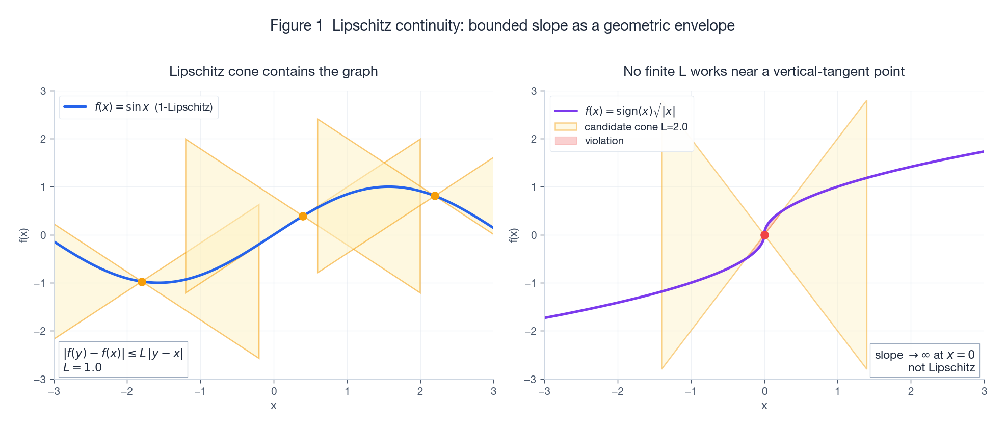
Left: $\sin x$ is 1-Lipschitz; the orange cones at three sample anchors fully contain the graph. Right: $\mathrm{sign}(x)\sqrt{|x|}$ has a divergent slope at the origin; the red region is where the candidate $L=2$ cone is pierced.
Two corollaries that will keep coming back:
- Uniform continuity: take $\delta = \varepsilon / L$.
- Closure: Lipschitz functions are closed under addition, scalar multiplication, and composition (constants multiply). This lets us decompose complicated models into Lipschitz building blocks with known constants.
1.2 Gradient-Lipschitz = $L$-smoothness
In practice we care less about Lipschitz $f$ and more about Lipschitz $\nabla f$, because that is what bounds the step size:
$$ \|\nabla f(y) - \nabla f(x)\| \le L\,\|y - x\|. $$A differentiable function satisfying this is called $L$-smooth. It admits a more practical equivalent statement, the descent lemma:
$$ \boxed{\,f(y) \le f(x) + \langle \nabla f(x), y - x\rangle + \frac{L}{2}\,\|y - x\|^2.\,} $$That is: $f$ is sandwiched from above by a family of upward parabolas with curvature $L$. The tangent line is the worst-case lower envelope; the parabola is the actual upper envelope.
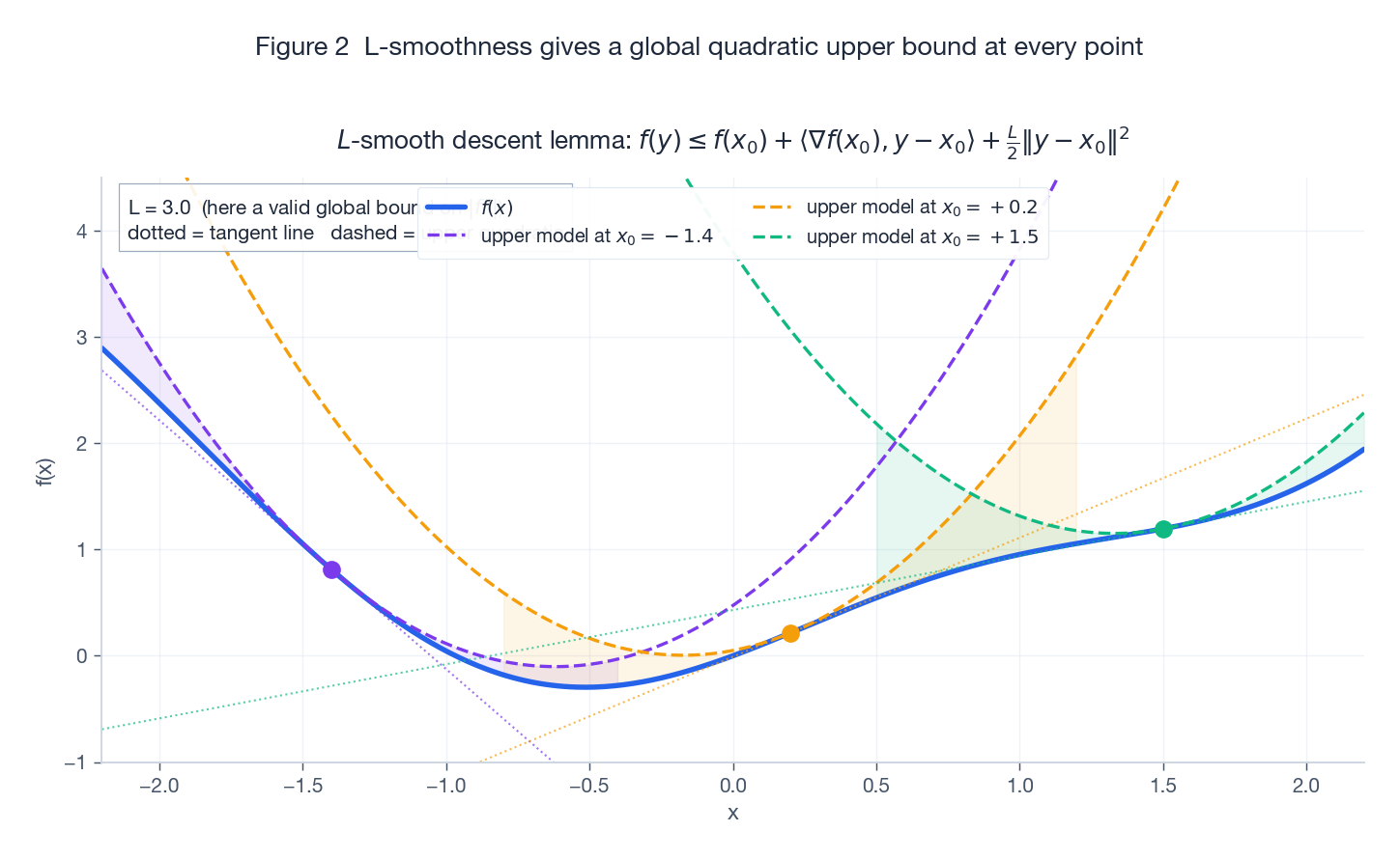
The blue curve is $f(x) = \tfrac{1}{2}\sin(2x) + \tfrac{1}{2}x^2$. At each of the three anchor points the dashed quadratic $f(x_0) + f'(x_0)(x-x_0) + \tfrac{L}{2}(x-x_0)^2$ stays above $f$ globally, while the dotted tangent line only stays below where $f$ is locally convex.
Why is this inequality so important? Plug $y = x - \eta\nabla f(x)$ into it:
$$ f(y) \le f(x) - \eta\Big(1 - \frac{L\eta}{2}\Big)\|\nabla f(x)\|^2. $$As long as $\eta \le 1/L$, the bracket is $\ge 1/2$, so every step strictly decreases $f$, with the decrease lower-bounded by a constant times $\|\nabla f\|^2$. This is the real origin of “step size at most $1/L$” — not folklore, but a direct corollary of the descent lemma.
1.3 Three worked examples
| Function | Gradient | Spectral norm of Hessian | $L$ |
|---|---|---|---|
| $\tfrac{1}{2}\|x\|^2$ | $x$ | $1$ | $1$ |
| $\tfrac{1}{2}\|Ax-b\|^2$ | $A^\top(Ax-b)$ | $\lambda_{\max}(A^\top A)$ | $\lambda_{\max}(A^\top A)$ |
| Logistic $\log(1 + e^{-y\,\theta^\top x})$ (one sample) | $-y\,\sigma(-y\theta^\top x)\,x$ | $\sigma(\cdot)\sigma(-\cdot)\,xx^\top$ | $\tfrac{1}{4}\|x\|^2$ |
The third row gives the standard $L = \tfrac{1}{4n}\sum_i\|x_i\|^2$ for logistic regression — the bound $\sigma(\cdot)\sigma(-\cdot)\le 1/4$ does the work.
1.4 Hessian spectral bound implies gradient Lipschitz
Theorem 1 (Hessian spectral norm $\Rightarrow$ Lipschitz gradient). If $f$ is twice differentiable with $\sup_x \|\nabla^2 f(x)\|_2 \le L$, then $\nabla f$ is $L$-Lipschitz.
Proof. By Newton-Leibniz,
$$ \nabla f(y) - \nabla f(x) = \int_0^1 \nabla^2 f(x + t(y-x))\,(y-x)\,\mathrm dt. $$Take 2-norms:
$$ \|\nabla f(y) - \nabla f(x)\| \le \int_0^1 \|\nabla^2 f(\cdot)\|_2\,\|y-x\|\,\mathrm dt \le L\,\|y-x\|.\quad\blacksquare $$For a quadratic $f(x) = \tfrac{1}{2}x^\top H x$ this gives $L = \lambda_{\max}(H)$ exactly — the same $L$ that the descent lemma uses, so the step rule $\eta \le 1/\lambda_{\max}(H)$ is tight.
2. Strong convexity: existence, uniqueness, quadratic growth
2.1 Three equivalent definitions
Definition ($\mu$-strongly convex). A differentiable $f$ is $\mu$-strongly convex ($\mu>0$) if for all $x, y$,
$$ f(y) \ge f(x) + \langle \nabla f(x), y - x\rangle + \frac{\mu}{2}\,\|y - x\|^2. $$It has three equivalent forms, each handier in a different context:
- Quadratic lower bound (the inequality above): $f$ sits above a family of upward parabolas with curvature $\mu$.
- $f - \tfrac{\mu}{2}\|x\|^2$ is convex: subtract off the “$\mu$-curvature mass” and you are left with a convex function.
- Second-order condition (if $f$ is $C^2$): $\nabla^2 f(x) \succeq \mu I$.
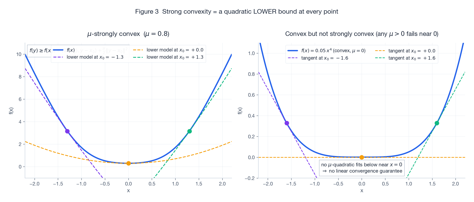
Left: a strongly convex function with three quadratic lower models (one per anchor). Right: $f(x) = 0.05\,x^4$ is convex but not strongly convex — it is too flat at the origin for any $\mu>0$ parabola to fit underneath. This is exactly why we cannot get linear convergence on this kind of objective.
2.2 Existence and uniqueness
Theorem 2 (existence). If $f$ is lower semi-continuous and some sublevel set $\{x : f(x)\le\alpha\}$ is non-empty and bounded, $f$ attains its minimum on that set.
This is just Weierstrass: closed + bounded = compact, and lsc functions attain their infimum on compact sets.
Theorem 3 (uniqueness from strong convexity). A $\mu$-strongly convex function ($\mu > 0$) on $\mathbb{R}^n$ has at most one global minimizer.
Proof. Suppose $x^\star, y^\star$ are both minimizers. Then $\nabla f(x^\star) = 0$, so the lower bound at $x = x^\star, y = y^\star$ gives
$$ f(y^\star) \ge f(x^\star) + 0 + \frac{\mu}{2}\|y^\star - x^\star\|^2. $$But $f(y^\star) = f(x^\star)$, so $\|y^\star - x^\star\| = 0$. $\blacksquare$
Corollary (PL / quadratic growth). Setting $x = x^\star$ in the lower bound,
$$ f(y) - f^\star \ge \frac{\mu}{2}\|y - x^\star\|^2, $$i.e. the cost grows at least quadratically away from the minimizer. This is the lever that turns “small function value” into “small distance to optimum” in every convergence proof below.
2.3 $L$-smooth and $\mu$-strongly convex together: the condition number
If $f$ satisfies both
$$ \mu I \preceq \nabla^2 f(x) \preceq L I, $$then all directional curvatures are squeezed into $[\mu, L]$. The ratio
$$ \boxed{\,\kappa := \frac{L}{\mu} \ge 1\,} $$is the condition number, and it controls every rate that follows. Large $\kappa$ means the function is “long and narrow” — the steepest direction is on the verge of instability while the flattest direction barely contributes any signal. That is the structural source of optimization difficulty.
3. Accelerated gradient descent: from $\kappa$ to $\sqrt{\kappa}$
3.1 Two upper bounds for plain GD
Theorem 4 (GD on convex + $L$-smooth, sublinear rate). Take $\eta = 1/L$:
$$ f(x_t) - f^\star \le \frac{L\,\|x_0 - x^\star\|^2}{2t} = \mathcal O(1/t). $$Theorem 5 (GD on $\mu$-strongly convex + $L$-smooth, linear rate). Take $\eta = 1/L$:
$$ \|x_t - x^\star\|^2 \le \Big(1 - \frac{1}{\kappa}\Big)^t \|x_0 - x^\star\|^2. $$Reaching error $\varepsilon$ takes $t = \mathcal O(\kappa\log(1/\varepsilon))$. The condition number enters linearly: on a least-squares problem with $\kappa = 10^4$, every additional factor of 10 in precision costs about another $2\times 10^4$ iterations.
3.2 Nesterov: lookahead trades $\kappa$ for $\sqrt{\kappa}$
Classical Polyak Heavy Ball is
$$ x_{t+1} = x_t - \alpha\nabla f(x_t) + \beta(x_t - x_{t-1}). $$It does hit the $\sqrt{\kappa}$ rate on strictly convex quadratics, but does not provably accelerate on general strongly convex functions — counterexamples blow it up. Nesterov’s key tweak is to evaluate the gradient at the lookahead point, not at $x_t$:
$$ \begin{aligned} y_t &= x_t + \beta_t (x_t - x_{t-1}), \\ x_{t+1} &= y_t - \eta\,\nabla f(y_t). \end{aligned} $$Intuition: take a momentum-extrapolated peek at where you are about to land, then correct using the gradient there. That bit of foresight is enough to preserve acceleration on every $L$-smooth convex function.
Theorem 6 (Nesterov, convex case, $\mathcal O(1/t^2)$). For $L$-smooth convex $f$, with $\eta = 1/L$ and the classical weights $\beta_t = (t-1)/(t+2)$,
$$ f(x_t) - f^\star \le \frac{2L\,\|x_0 - x^\star\|^2}{(t+1)^2}. $$Theorem 7 (Nesterov, strongly convex case, $\mathcal O((1 - 1/\sqrt{\kappa})^t)$). For $\mu$-strongly convex + $L$-smooth $f$, with $\eta = 1/L$ and constant momentum
$$ \beta = \frac{1 - \sqrt{1/\kappa}}{1 + \sqrt{1/\kappa}}, $$we get $f(x_t) - f^\star \le \big(1 - \sqrt{1/\kappa}\big)^t (f(x_0) - f^\star)$, hence $t = \mathcal O(\sqrt{\kappa}\log(1/\varepsilon))$.
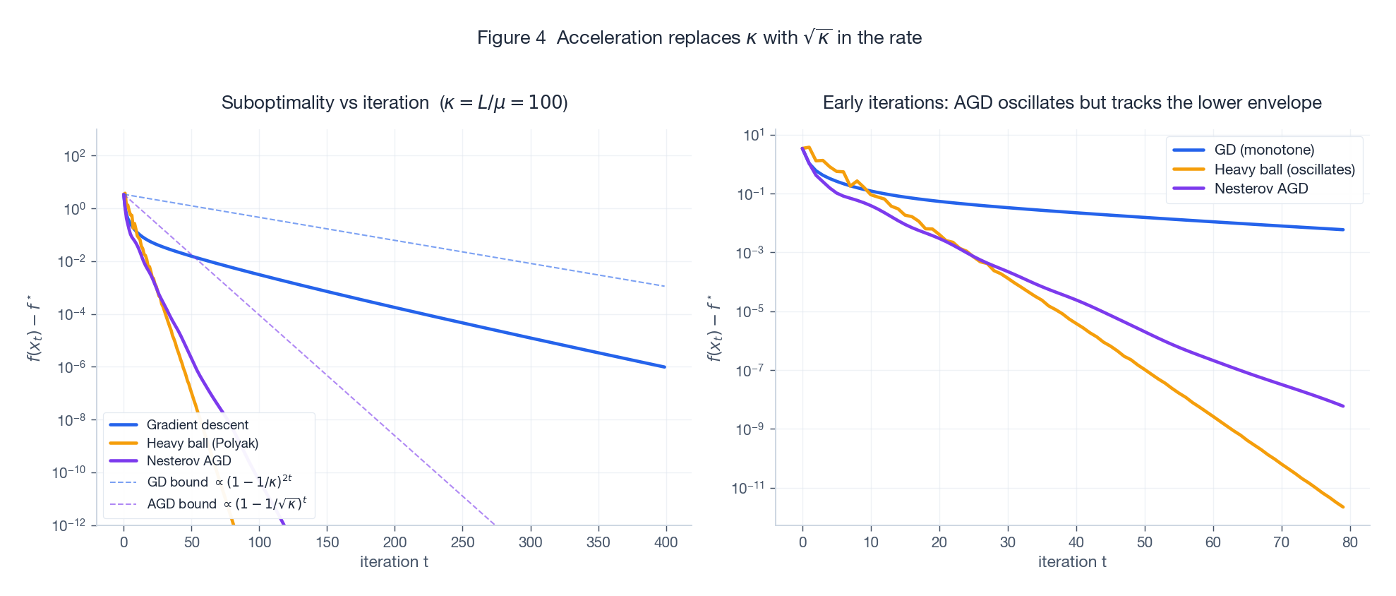
Left ($\kappa=100$): on a log axis all three algorithms decrease linearly, but Nesterov (purple) and Heavy Ball (orange) have a steeper slope than GD (blue) — that is the $\sqrt{\kappa}$ vs $\kappa$ gap made visible. The dashed lines are the theoretical envelopes; they match the empirical traces. Right: zoom in on the first 80 iterations and Nesterov is non-monotone — it oscillates inside the lower envelope. That is the price of acceleration.
3.3 Adaptive restart fixes the side effects of acceleration
Acceleration’s downside is non-monotonicity — the function value bumps up periodically. This becomes painful in two situations:
- $\mu$ unknown: Theorem 7 needs $\sqrt{1/\kappa}$ in the momentum; misestimating it kills the rate.
- Locally strongly convex: $f$ is only globally convex but strongly convex near $x^\star$; the convex-rate Nesterov underperforms.
Adaptive restart (O’Donoghue & Candès, 2015): whenever the gradient direction reverses ($\langle\nabla f(y_t), x_{t+1}-x_t\rangle > 0$) or the function value rises, reset the momentum and the iteration counter $t \leftarrow 1$.
Theorem 8 (restart Nesterov hits the optimal rate without knowing $\mu$). For $\mu$-strongly convex + $L$-smooth $f$, restart Nesterov still achieves $\mathcal O(\sqrt{\kappa}\log(1/\varepsilon))$ iterations, without needing $\mu$.
Proof sketch: between two restarts, you run convex-rate Nesterov, so the gap drops as $\mathcal O(1/k^2)$. Combined with the quadratic-growth corollary, this gives “each restart at least halves the gap.” A geometric halving $\log(1/\varepsilon)$ times reaches $\varepsilon$. Each segment has length $\sim \sqrt{\kappa}$, so total iterations are $\sim \sqrt{\kappa}\log(1/\varepsilon)$.
3.4 How much does $\kappa$ actually matter
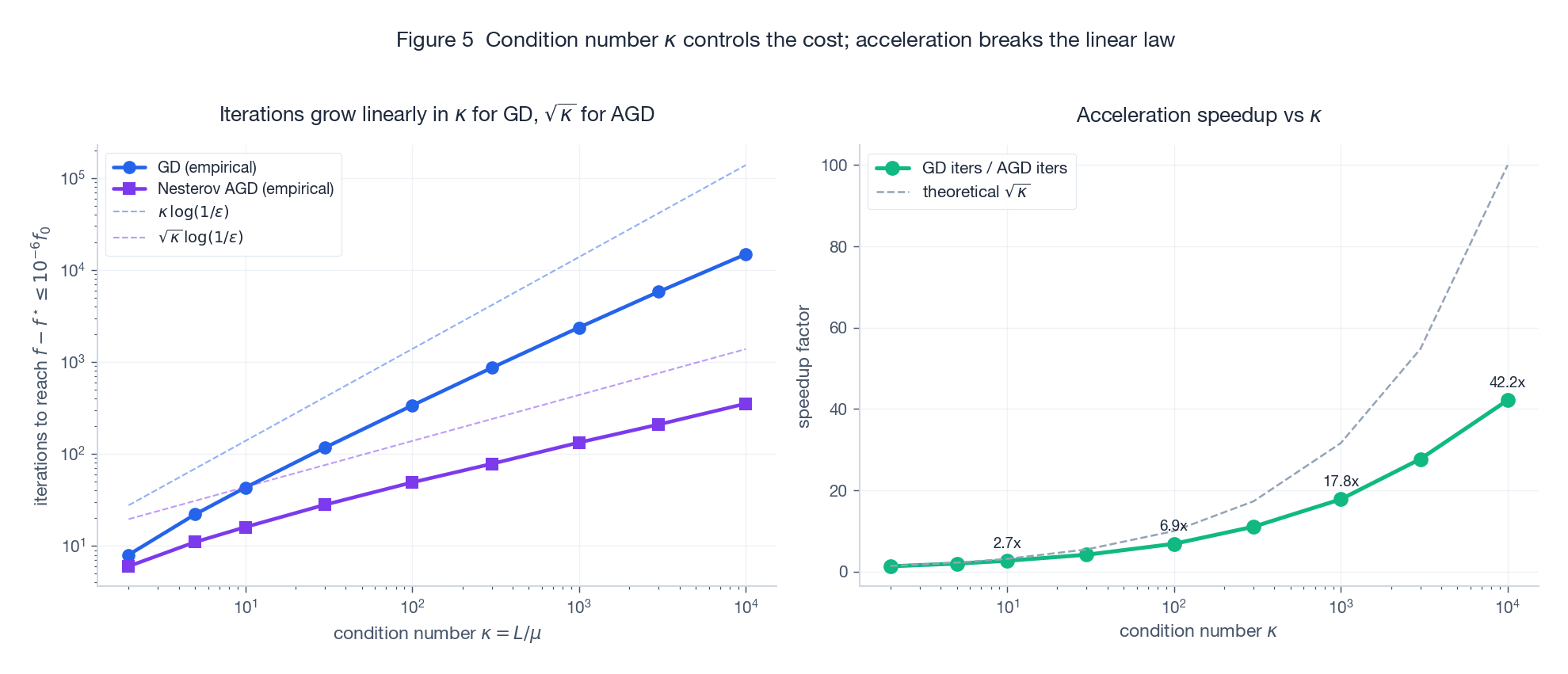
Left (log-log): on synthetic least squares, the iterations to reach $10^{-6}$ relative gap grow strictly along $\kappa$ for GD and along $\sqrt{\kappa}$ for Nesterov. Right: the speedup ratio $T_{\text{GD}}/T_{\text{AGD}}$ tracks $\sqrt{\kappa}$ almost exactly. At $\kappa = 10^4$ the speedup is ~100x; at $\kappa = 100$ it is ~10x. The worse the conditioning, the more acceleration pays off.
3.5 A decision table
| Situation | Recommendation | Why |
|---|---|---|
| Small $\kappa$ ($\le 50$), keep code simple | GD | Acceleration’s complexity payoff is small |
| Large $\kappa$, $\mu$ known | Constant-momentum Nesterov (Thm 7) | Closed-form optimal $\beta$ |
| Large $\kappa$, $\mu$ unknown / locally s.c. | Adaptive-restart Nesterov | Adapts to $\mu$ while keeping the optimal rate |
| Strictly convex quadratic (least squares) | Conjugate Gradient first | Finite termination in $\le n$ steps, beats Nesterov |
| Non-convex but locally near-convex (deep nets) | Momentum / Adam with warmup + cosine | Theoretical rates no longer provable; engineering rules dominate |
4. The least-squares experiment
4.1 Problem and exact constants
Consider
$$ \min_{x\in\mathbb{R}^n} f(x) = \frac{1}{2}\|Ax - b\|^2, \qquad A\in\mathbb{R}^{m\times n},\; b\in\mathbb{R}^m. $$Differentiate:
$$ \nabla f(x) = A^\top(Ax - b), \qquad \nabla^2 f(x) = A^\top A, $$so
$$ L = \lambda_{\max}(A^\top A), \qquad \mu = \lambda_{\min}(A^\top A), \qquad \kappa = \kappa(A^\top A) = \kappa(A)^2. $$Critical caveat. The condition number is the square of $A$’s condition number. So an $A$ that “looks fine” with $\kappa(A) = 100$ becomes a hard $\kappa = 10^4$ instance for least squares — and for the normal-equation gradient, no less.
4.2 Implementation
| |
4.3 What we observe
On a synthetic instance with $m = 200, n = 100$, $\kappa(A) \approx 100$ (so $\kappa(A^\top A) \approx 10^4$):
- GD: needs ~$4\times 10^4$ iterations to reach $10^{-6}$ relative gradient norm; smooth but slow.
- Nesterov (constant momentum): ~400 iterations; the trace oscillates inside the trough as Figure 4 (right) predicts.
- Restart Nesterov: ~500 iterations and almost perfectly monotone — the most robust of the three.
The empirical speedup matches the $\sqrt{\kappa}$ prediction from Figure 5 ($10^4 \to 100\times$).
5. Summary and where to go next
5.1 The cheat sheet
| Assumption | Algorithm | Rate | Step size |
|---|---|---|---|
| $L$-smooth, convex | GD | $\mathcal O(1/t)$ | $\eta = 1/L$ |
| $L$-smooth, $\mu$-strongly convex | GD | $\big(1 - 1/\kappa\big)^t$ | $\eta = 1/L$ |
| $L$-smooth, convex | Nesterov | $\mathcal O(1/t^2)$ | $\eta = 1/L,\ \beta_t = (t-1)/(t+2)$ |
| $L$-smooth, $\mu$-strongly convex | Nesterov | $\big(1 - 1/\sqrt{\kappa}\big)^t$ | $\eta = 1/L,\ \beta = (1-\sqrt{1/\kappa})/(1+\sqrt{1/\kappa})$ |
| Same, $\mu$ unknown | Restart Nesterov | $\big(1 - 1/\sqrt{\kappa}\big)^t$ | adaptive |
5.2 Three reflexes for any new problem
When a fresh objective lands on your desk, walk this loop:
- How steep? Estimate $L$ (largest eigenvalue or backtracking line search). It immediately gives you the step ceiling.
- How sharp at the bottom? Estimate $\mu$ (smallest eigenvalue or a PL constant). It tells you whether linear convergence is on the table.
- Is acceleration worth it? Look at $\kappa = L/\mu$. $\kappa < 50$: GD is fine. $\kappa \in [50, 10^4]$: switch to Nesterov. $\kappa > 10^4$: think about preconditioning or a second-order method.
5.3 Where the story continues
- Non-convex + PL condition. Drop strong convexity; if $\tfrac{1}{2}\|\nabla f\|^2 \ge \mu(f - f^\star)$ holds, GD still converges linearly. This is the theoretical seed of “why over-parameterised deep nets train linearly” (Karimi et al., 2016).
- Acceleration with noise. Vanilla Nesterov is not robust to stochastic gradients. SAG / SVRG / Katyusha pull the strongly-convex stochastic rate back to the $\sqrt{\kappa}$ regime through variance reduction.
- Second-order acceleration. Sophia and Shampoo precondition by a (block-)diagonal Hessian, effectively rewriting the condition number — an active 2024 frontier in large-scale pretraining.
References
- Nesterov, Y. (1983). A method of solving a convex programming problem with convergence rate $\mathcal O(1/k^2)$. Soviet Mathematics Doklady, 27(2), 372–376.
- Boyd, S., & Vandenberghe, L. (2004). Convex Optimization. Cambridge University Press.
- Bubeck, S. (2015). Convex Optimization: Algorithms and Complexity. Foundations and Trends in Machine Learning, 8(3-4), 231–357.
- O’Donoghue, B., & Candès, E. (2015). Adaptive restart for accelerated gradient schemes. Foundations of Computational Mathematics, 15(3), 715–732.
- Karimi, H., Nutini, J., & Schmidt, M. (2016). Linear convergence of gradient and proximal-gradient methods under the Polyak-Łojasiewicz condition. ECML-PKDD.