Why is “tuning the LR is an art” a meme for ResNet, while every modern LLM paper just writes “AdamW, $\beta_1{=}0.9, \beta_2{=}0.95, \mathrm{wd}{=}0.1$” and moves on? It is not an accident — it is the end-point of three decades of optimizer evolution.

This post walks the lineage end-to-end on a single thread: each step exists because of a specific failure of the previous one. We end with the three directions that have actually entered the post-2023 large-model toolkit: Lion, Sophia, and Schedule-Free.

What you will learn

Why GD zig-zags on ill-conditioned losses, and how momentum fixes it physically
The exact mathematical difference between Nesterov “lookahead” and classical momentum
Why AdaGrad is a killer on sparse features, and why it eventually “suffocates” in deep nets
How RMSProp rescued AdaGrad with a one-line change (exponential moving average)
How Adam stitches momentum and RMSProp together, and why bias correction matters
AdamW vs Adam: why “L2 == weight decay” stops being true once you put adaptive scaling in the denominator
Lion / Sophia / Schedule-Free: the three post-AdamW directions that scaled

Prerequisites

Basic calculus (gradients, Hessian, Taylor expansion)
Some experience training a neural network (any framework)

The lineage at a glance

Year	Algorithm	Specific problem it fixed
1847	GD	Formalized “step along the negative gradient”
1951	SGD	Datasets too big for full-batch gradients
1964	Momentum	GD zig-zags in narrow valleys
1983	NAG	Plain momentum overshoots near minima
2011	AdaGrad	Sparse features need per-coordinate LRs
2012	RMSProp	AdaGrad’s denominator suffocates the LR
2014	Adam	Combine direction (momentum) and scale (RMSProp)
2017	AdamW	Adam + L2 != Adam + weight decay
2023	Lion	Drop the second moment; use sign of momentum
2023	Sophia	Cheap diagonal-Hessian preconditioner
2024	Schedule-Free	Stop needing to know the total step count

The sections below follow this order.

1. Gradient descent (GD): the origin

Given a differentiable loss $J(\theta)$, the simplest update is

$$ \theta_{t+1} = \theta_t - \eta\,\nabla J(\theta_t). $$

Convergence: if $J$ is convex with $L$-Lipschitz gradient, $\eta \le 1/L$ guarantees (sub)linear convergence to the global minimum.

The fatal weakness that motivates everything else:

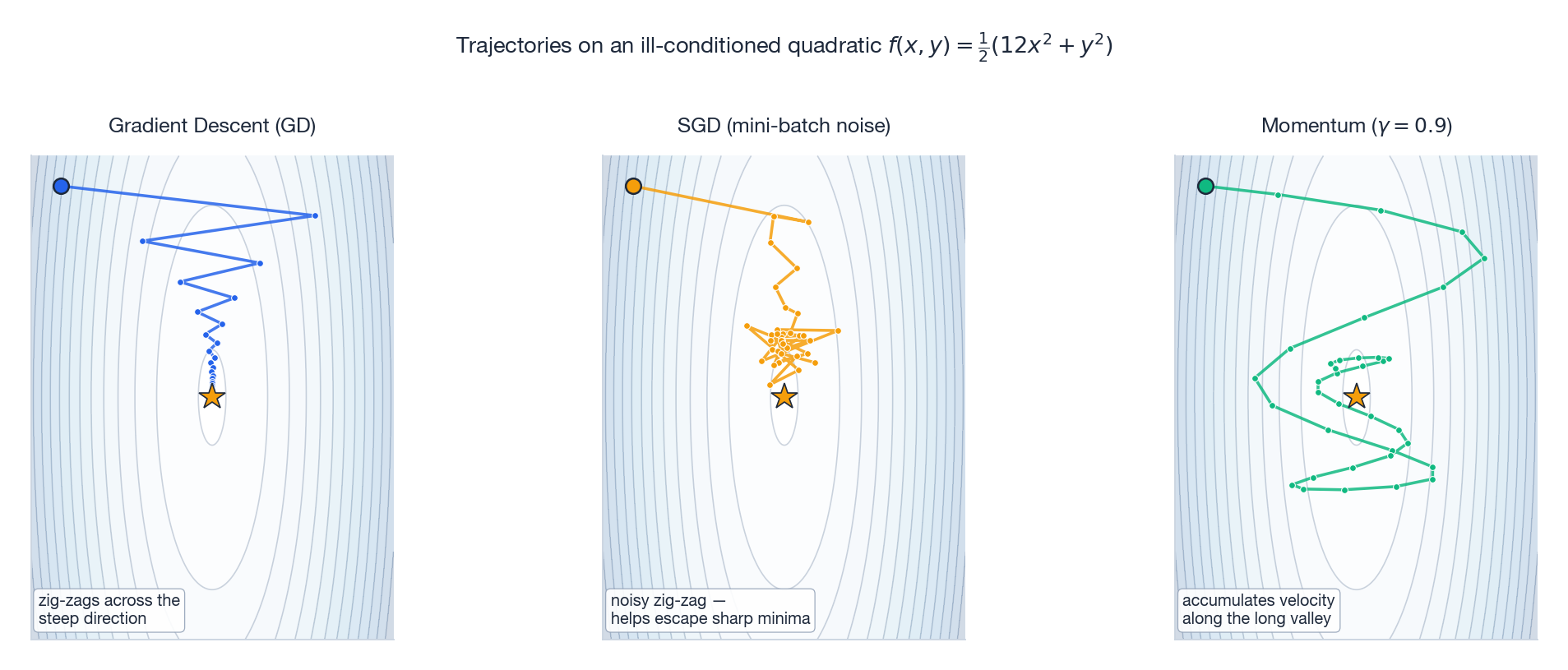
Under ill-conditioned curvature (Hessian condition number $\kappa = \lambda_{\max}/\lambda_{\min}$ large), the iteration count grows linearly in $\kappa$. The 1-D intuition: $f(\theta)=\frac{1}{2}H\theta^2$ gives $\theta_{t+1}=(1-\eta H)\theta_t$, stable iff $\eta < 2/H$. Your step is capped by the curvature in the steepest direction.
When the steepest direction ($\lambda_{\max}$) and the flattest direction ($\lambda_{\min}$) differ by orders of magnitude, you barely move along the flat one but bounce back and forth along the steep one. That is the narrow-valley problem — visible in the left panel of Fig 1 below.

2. SGD: the price and bonus of noise

Once datasets do not fit in memory, you replace the full gradient with a mini-batch estimate:

$$ g_t = \nabla J(\theta_t) + \xi_t,\qquad \mathbb{E}[\xi_t]=0. $$

The noise $\xi_t$ is both a curse and a blessing:

Curse: a slightly larger step gets amplified by noise into divergence.
Blessing: noise helps escape sharp local minima — later linked by Keskar et al. to the “flat-minima” generalization story.

Fig 1 middle panel: SGD’s trajectory in the same valley is hairier than GD’s, but on average it still flows toward the bottom.

3. Momentum: give the optimizer some inertia

Mental model: think of $\theta$ as a ball rolling down the valley. GD is a “massless bug” — every step only sees the local slope, so it bounces around the narrow direction. Give the bug some mass and inertia accumulates along the long axis of the valley while the perpendicular bounces cancel out.

$$ v_t = \gamma v_{t-1} + \eta\,g_t,\qquad \theta_{t+1} = \theta_t - v_t. $$

Typical $\gamma = 0.9$ — geometrically weights past gradients with effective memory $\approx 1/(1-\gamma) = 10$ steps.

Key insight: momentum amplifies the effective step size by roughly $1/(1-\gamma)$. So when you turn momentum on, you must shrink the LR you used without it. This is the most common beginner trap.

Fig 1 right panel: the same valley, but momentum’s path is “straightened” — perpendicular oscillation cancels, longitudinal velocity accumulates.

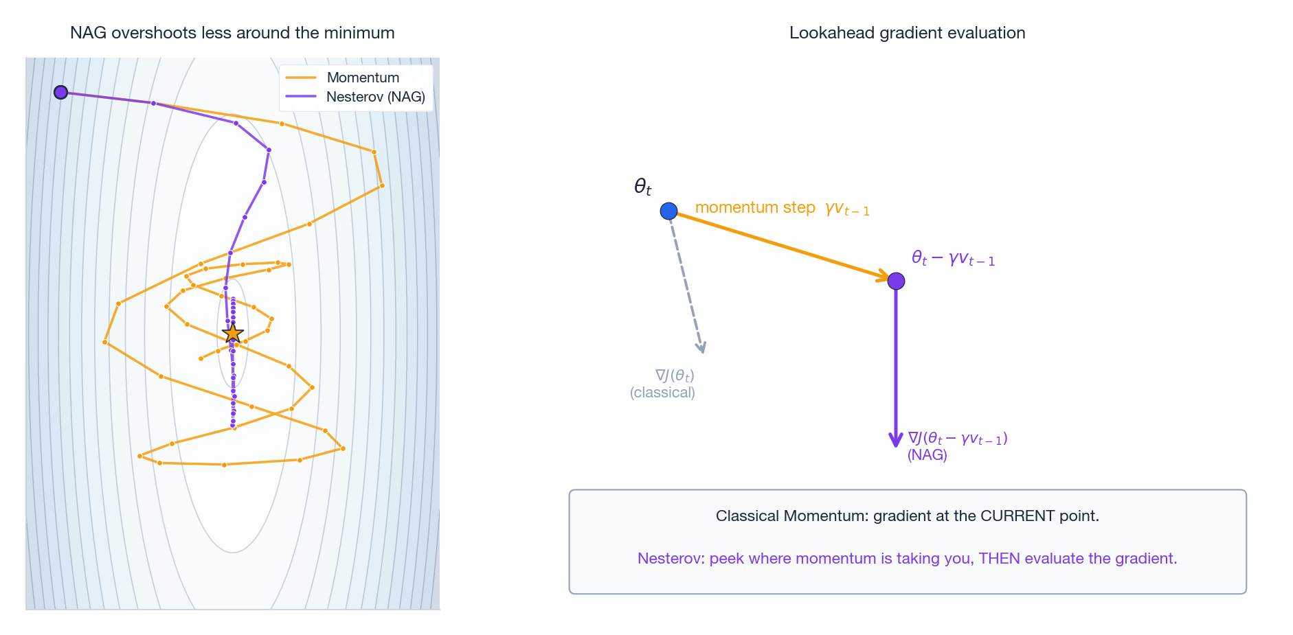
GD / SGD / Momentum trajectories on an ill-conditioned quadratic

4. Nesterov accelerated gradient (NAG): peek before you leap

Classical momentum overshoots near the minimum: it computes the gradient at the current point, so it only learns “oops, I went too far” one step too late.

NAG changes one line:

$$ v_t = \gamma v_{t-1} + \eta\,\nabla J(\theta_t - \gamma v_{t-1}),\qquad \theta_{t+1} = \theta_t - v_t. $$

The only difference is where you evaluate the gradient: classical momentum at $\theta_t$, NAG at the lookahead point $\theta_t - \gamma v_{t-1}$ — i.e. “where the momentum step alone would have taken me”.

Why it works: it is a one-step look-ahead. If the slope is about to flatten, NAG sees that early and decelerates; the converse for steepening. Nesterov (1983) proved this accelerates convex smooth optimization from $O(1/t)$ to $O(1/t^2)$.

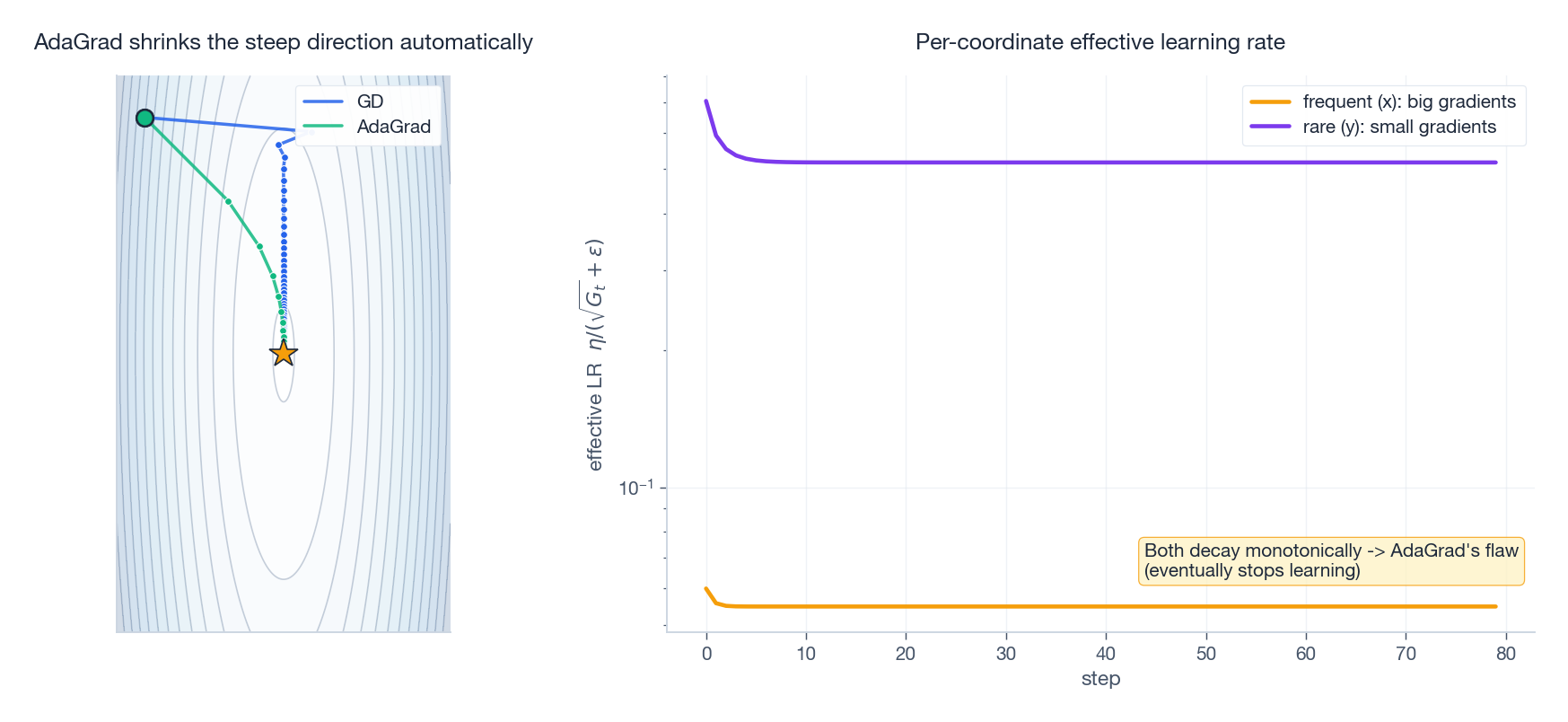
NAG: lookahead gradient evaluation reduces overshoot

5. AdaGrad: every coordinate gets its own learning rate

By 2011, NLP was drowning in sparse features — think word2vec where a rare word might appear 5 times in a million examples. With a single $\eta$ for everything:

Rare-word parameters: small gradients, but the same $\eta$ is either too big (kills them) or too small (they never learn).
Frequent-word parameters: big and frequent gradients, would prefer smaller steps.

Duchi proposed AdaGrad — per-coordinate adaptation based on each coordinate’s own gradient history:

$$ G_t = G_{t-1} + g_t^2 \quad(\text{element-wise}) $$$$ \theta_{t+1} = \theta_t - \frac{\eta}{\sqrt{G_t}+\epsilon}\,g_t. $$

Intuition: large accumulated $g^2$ -> large denominator -> small effective step. Rare-but-suddenly-large coordinate -> small denominator -> large effective step. LR is auto-distributed by frequency.

The fatal flaw: $G_t$ is a monotonically growing sum. Train deep nets for hundreds of thousands of steps and the denominator drives every effective LR toward zero. The model “suffocates”. The right panel of Fig 3 makes this concrete.

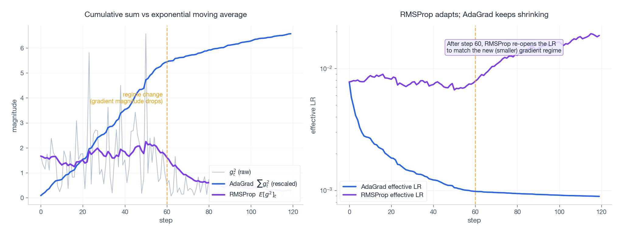
AdaGrad: shrinks the steep direction automatically, but every per-coord LR decays monotonically

6. RMSProp: replace cumulative sum with EMA

In his 2012 Coursera slides, Hinton changed exactly one thing and rescued AdaGrad: replace the cumulative sum $\sum g_t^2$ with an exponential moving average:

$$ E[g^2]_t = \rho\,E[g^2]_{t-1} + (1-\rho)\,g_t^2 $$$$ \theta_{t+1} = \theta_t - \frac{\eta}{\sqrt{E[g^2]_t}+\epsilon}\,g_t. $$

Typical $\rho = 0.9$ — “remember roughly the last 10 steps of gradient magnitude”.

The crucial difference:

AdaGrad: $G_t$ only ever grows -> LR only ever shrinks (irreversible).
RMSProp: $E[g^2]_t$ is a finite-window average -> when gradient magnitude changes, the denominator follows -> the LR can scale back up.

Fig 4 right panel shows this directly: at step 60 the gradient magnitude drops sharply. AdaGrad’s effective LR keeps falling; RMSProp’s effective LR climbs back to match the new regime.

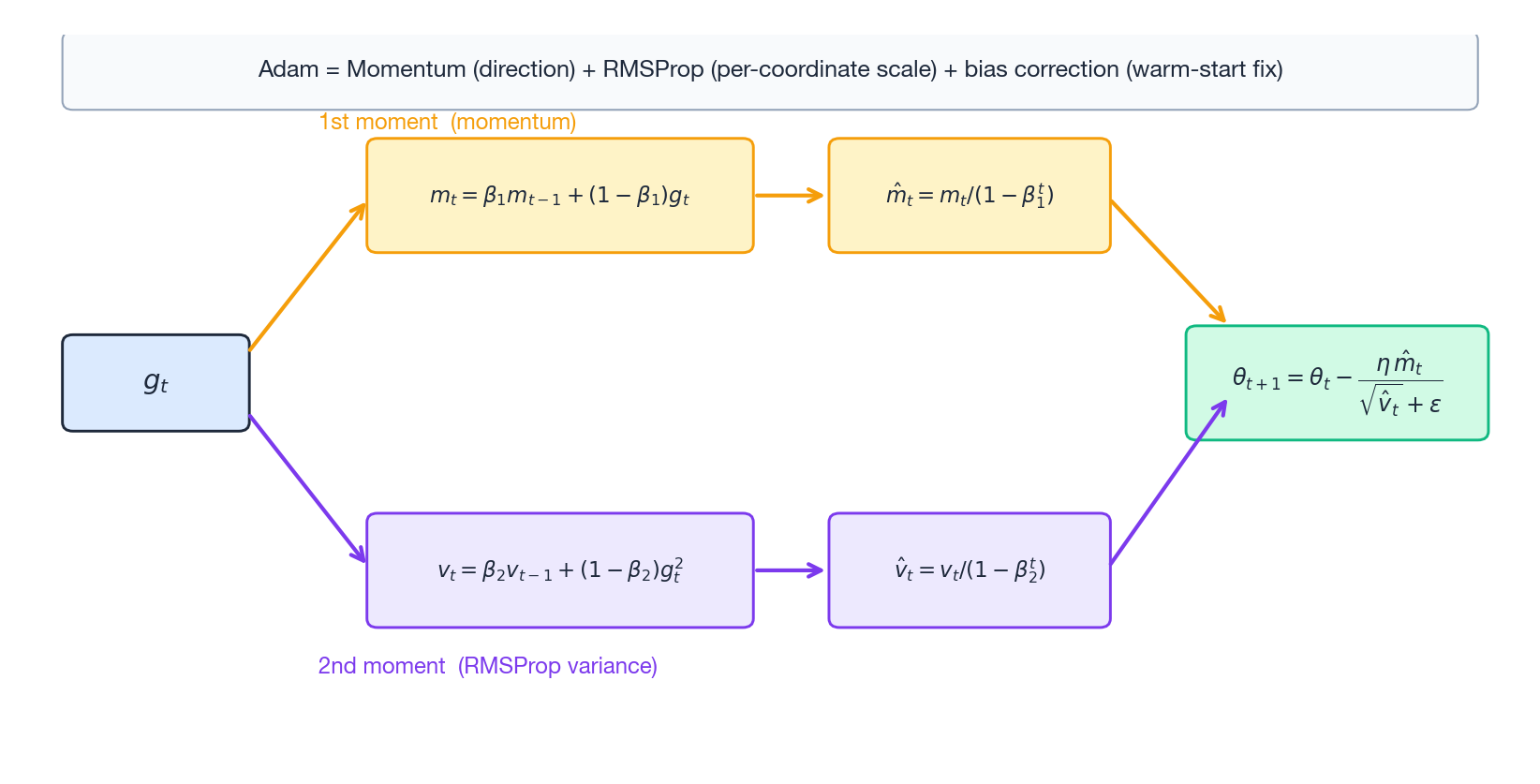
RMSProp (EMA) vs AdaGrad (cumulative) under non-stationary gradient magnitude

7. Adam: stitch momentum and RMSProp together

By now both threads were mature:

Momentum gives a good direction.
RMSProp gives a good per-coordinate scale.

Kingma & Ba (2014) just bolted them together:

$$ m_t = \beta_1 m_{t-1} + (1-\beta_1)\,g_t \quad\text{(1st moment = momentum)} $$$$ v_t = \beta_2 v_{t-1} + (1-\beta_2)\,g_t^2 \quad\text{(2nd moment = RMSProp)} $$

Bias correction — the most under-appreciated detail. Because $m_0=v_0=0$, both $m_t$ and $v_t$ are heavily biased toward zero in the first few steps. Fix:

$$ \hat m_t = \frac{m_t}{1-\beta_1^t},\qquad \hat v_t = \frac{v_t}{1-\beta_2^t} $$$$ \theta_{t+1} = \theta_t - \frac{\eta\,\hat m_t}{\sqrt{\hat v_t}+\epsilon}. $$

Defaults: $\beta_1 = 0.9,\ \beta_2 = 0.999,\ \epsilon = 10^{-8}$.

Why $\beta_2$ is much larger than $\beta_1$: variance estimates are noisier than mean estimates and need a longer averaging window. $1/(1-0.999) = 1000$ steps — and that is exactly why Adam typically needs ~1000 warmup steps before $v_t$ “warms up”.

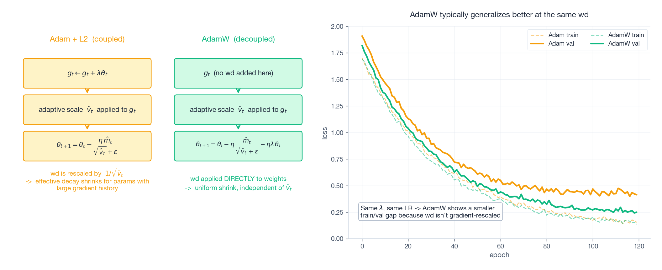
Adam dataflow: momentum branch + RMSProp branch -> bias correction -> adaptive update

8. AdamW: the weight-decay bug that lived for a decade

Adding L2 regularization $\frac{\lambda}{2}\|\theta\|^2$ to the loss adds a term $\lambda\theta$ to the gradient. In SGD this is exactly equivalent to multiplying weights by $(1-\eta\lambda)$ each step — the classical “weight decay”.

But Loshchilov & Hutter (2017) noticed that in Adam these two operations are no longer equivalent. The reason is direct: Adam divides the gradient by $\sqrt{\hat v_t}$. If you fold $\lambda\theta$ into the gradient, it also gets divided by $\sqrt{\hat v_t}$ — meaning parameters with large gradient history get less weight decay, which is the opposite of what regularization wants.

AdamW’s fix is to take weight decay out of the gradient and apply it directly to the parameters:

$$ \theta_{t+1} = \theta_t - \eta\,\frac{\hat m_t}{\sqrt{\hat v_t}+\epsilon} - \eta\lambda\,\theta_t. $$

The effect: at the same $\lambda$ and LR, AdamW’s generalization gap on ImageNet/Transformer is meaningfully smaller than Adam+L2. This is why post-2018 every large-model pretrain defaults to AdamW.

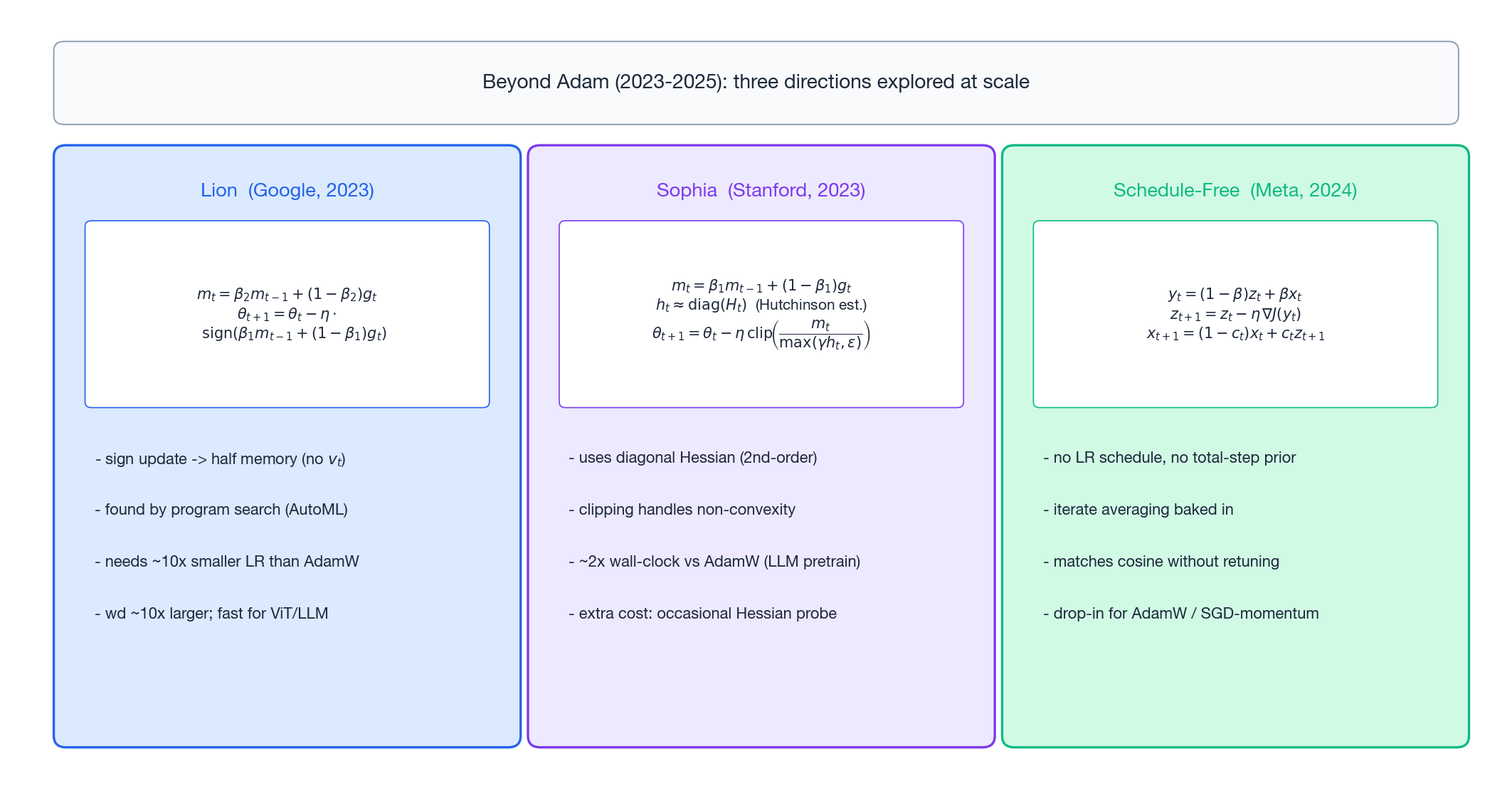
AdamW (decoupled) vs Adam+L2 (coupled): where weight decay enters the update

9. The post-2023 frontier: three directions that scaled

After AdamW reigned for ~6 years, three directions have actually proven themselves at scale since 2023.

9.1 Lion (Google, 2023): only the sign

Discovered by AutoML program search; the update keeps only the sign:

$$ m_t = \beta_2 m_{t-1} + (1-\beta_2)\,g_t $$$$ \theta_{t+1} = \theta_t - \eta\,\mathrm{sign}\bigl(\beta_1 m_{t-1} + (1-\beta_1)\,g_t\bigr). $$

Notable properties:

Half the optimizer state: no $v_t$ needed — meaningful real money for hundred-billion-parameter models.
Constant update magnitude $\eta$: because sign returns $\pm 1$. So Lion’s LR must be about 10x smaller than AdamW’s, and wd about 10x larger.
On ViT and LLM pretraining, matches or slightly beats AdamW with faster wall-clock.

9.2 Sophia (Stanford, 2023): cheap second-order

Sophia plugs a cheap diagonal-Hessian estimate into the denominator:

$$ m_t = \beta_1 m_{t-1} + (1-\beta_1)\,g_t $$$$ h_t \approx \mathrm{diag}(H_t) \quad\text{(Hutchinson estimate, every } k \text{ steps)} $$$$ \theta_{t+1} = \theta_t - \eta\,\mathrm{clip}\!\left(\frac{m_t}{\max(\gamma h_t,\,\varepsilon)},\,1\right). $$

Core tricks:

Use $\mathrm{diag}(H)$ instead of $g^2$ as the denominator — that is the actual curvature.
The clip is essential: $h_t$ can be negative in non-convex losses, and clipping keeps the update bounded.
The Hessian probe runs only every $k$ steps, so amortized cost is modest.

Reported results: roughly halves the wall-clock to reach a given perplexity at GPT-2 scale.

9.3 Schedule-Free (Meta, 2024): drop the schedule

LR schedules (cosine, WSD, etc.) all share one annoyance: you must know the total step count in advance. During research you usually do not, so committing to a schedule ties your hands.

Schedule-Free AdamW replaces the schedule with iterate averaging:

$$ y_t = (1-\beta) z_t + \beta x_t \quad\text{(point at which the gradient is taken)} $$$$ z_{t+1} = z_t - \eta\,\nabla J(y_t) $$$$ x_{t+1} = (1-c_t)\,x_t + c_t\,z_{t+1} \quad\text{(returned "averaged" parameters)} $$

The result: matches the final performance of cosine schedules without any explicit decay, and can be extended mid-training without redesigning anything.

Lion / Sophia / Schedule-Free: the three post-AdamW directions

10. Selection guide

Setting	Recommendation	Why
Convex / simple regression	GD or SGD-momentum	Strong theory, easy tuning
CV baseline	SGD + Nesterov + cosine	Historically the best optimum on ResNet/CNN
Transformer / LLM pretraining	AdamW + warmup + cosine/WSD	Industry default; close to free lunch
Memory-constrained large models	Lion	Saves the 1st-moment-equivalent state (~1/3 memory)
Research, unknown training length	Schedule-Free AdamW	Extend mid-run, no schedule redesign
Chasing wall-clock SOTA	Sophia	2nd-order acceleration, but engineering cost

11. Five facts that get missed most often

If you turn momentum on, lower the LR. Momentum amplifies the effective step by roughly $1/(1-\gamma)$. With $\gamma=0.9$ that is ~10x.
Adam’s $\beta_2 = 0.999$ implies a ~1000-step warmup because $v_t$ has not “warmed up” before that.
AdamW’s wd is decoupled from the LR. When the LR scheduler decays the LR, wd does NOT decay with it. This is the fundamental difference from the old SGD+L2 workflow.
Lion’s LR must be ~10x smaller than AdamW’s. Copy-pasting AdamW’s 3e-4 will diverge immediately.
Second-order methods looked “permanently impractical” not because they are bad, but because Hessians used to be too expensive. Sophia broke that wall by combining $\mathrm{diag}(H)$ with cheap Hutchinson estimation.

Summary

Three decades of optimizer evolution compress to two sentences:

GD to Adam: first solve the direction problem (momentum), then the scale problem (AdaGrad / RMSProp), then merge them and fix the bias (Adam).
Adam onwards: algorithmic improvement gives way to regularization detail (AdamW), memory efficiency (Lion), second-order information (Sophia), and schedule freedom (Schedule-Free).

If you only remember one thing: the LLM-era default is still AdamW + warmup + cosine/WSD + gradient clipping. Until you have a concrete bottleneck (memory, wall-clock, schedule flexibility), every paper claiming to beat AdamW deserves a baseline reproduction on your own task before you commit.

Optimizer Evolution: From Gradient Descent to Adam (and Beyond, 2025)