Proximal Operator: From Moreau Envelope to ISTA/FISTA and ADMM
A systematic walk through the proximal operator: convex-analysis basics, the Moreau envelope, closed-form proxes, and how they power ISTA, FISTA, ADMM, LASSO, and SVM in practice.
When your objective contains a non-smooth piece (sparse regularisation, total variation, an indicator of a constraint set) or a constraint that is hard to handle directly, “just do gradient descent” stalls – there is no gradient at the kink, or every step violates feasibility. The proximal operator is the engineered, beautiful workaround: think of each update as “take a step on the smooth part, then run a tiny penalised minimisation that pulls the iterate back toward a structured solution”.
This guide builds the minimum convex-analysis toolkit, derives the Moreau envelope and the core properties of the prox map, lists the closed-form proxes you actually use, and plugs them into ISTA, FISTA, ADMM, SVM, and sparse optimisation – with an emphasis on why each piece works, when one method beats another, and the implementation traps that hurt the most.
What you will learn
- Minimum convex-analysis toolkit: convex sets, convex functions, subgradients
- The proximal operator: definition, geometric intuition, four core properties
- Three closed-form proxes you will reach for daily: soft-threshold, projection, quadratic shrinkage
- The Moreau envelope: how it smooths a non-smooth function, and the gradient identity that drives ISTA
- ISTA: the smallest possible proximal-gradient algorithm
- FISTA: momentum acceleration to $O(1/k^2)$
- LASSO end-to-end: from theory to a clean Python implementation
- ADMM in one page, and how it relates to the prox-gradient family
- Common implementation traps: step-size, Lipschitz estimation, convergence checks
Prerequisites
- Multivariable calculus (gradient, chain rule)
- Linear algebra basics (norms, inner products, eigenvalues)
- A bit of convex-optimisation common sense (gradient descent, strong convexity)
Convex-Analysis Foundations
Before getting to the prox we need to settle three pieces – convex sets, convex functions, subgradients. Every property that follows (non-expansiveness, closed-form solutions, convergence rates) rests on them.
Convex sets and convex functions
Convex set: $C \subseteq \mathbb{R}^n$ is convex iff for any $x, y \in C$ and $\theta \in [0, 1]$,
$$\theta x + (1 - \theta) y \in C.$$The line segment between any two points stays in $C$.
Convex function: $f : \mathbb{R}^n \to \mathbb{R} \cup \{+\infty\}$ is convex iff its effective domain $\mathrm{dom}\,f$ is convex and for any $x, y \in \mathrm{dom}\,f$ and $\theta \in [0, 1]$,
$$f\!\left(\theta x + (1 - \theta) y\right) \le \theta f(x) + (1 - \theta) f(y).$$Geometrically, the chord above any two points sits above the function (“cup-shaped”).
Two facts to keep in your head:
- Local minimum is global minimum for a convex function.
- Supporting hyperplanes exist at every boundary point of a convex set, and at every point of a convex function – this is exactly where subgradients come from.
Subgradients
A differentiable convex function has a unique gradient $\nabla f(x)$ everywhere. Functions like $|x|$ or hinge $\max(0, 1 - t)$ have kinks – no gradient at the kink. We need subgradients.
Definition: $g \in \mathbb{R}^n$ is a subgradient of a convex $f$ at $x$ iff for any $y$,
$$f(y) \ge f(x) + \langle g,\, y - x \rangle.$$That is, $g$ defines a supporting hyperplane lying below the graph of $f$ that touches $f$ at $x$. The set of all such $g$ is the subdifferential $\partial f(x)$.
Worked example (absolute value): take $f(t) = |t|$.
$$ \partial |t| = \begin{cases} \{+1\}, & t > 0,\\ \{-1\}, & t < 0,\\ [-1, +1], & t = 0. \end{cases} $$At $t = 0$ the subdifferential is an interval – exactly the source of the soft-threshold’s “dead zone” later on.
Properties:
- If $f$ is differentiable at $x$, then $\partial f(x) = \{\nabla f(x)\}$.
- $\partial f(x)$ is always a convex set (and non-empty in the interior of $\mathrm{dom}\,f$ when $f$ is closed proper convex).
- Optimality condition: $x^\star$ is a global minimum of $f$ iff $0 \in \partial f(x^\star)$. This generalises “gradient = 0” and is the workhorse of every derivation below.
The Proximal Operator
Definition and geometric intuition
For a closed proper convex function $f : \mathbb{R}^n \to \mathbb{R} \cup \{+\infty\}$ and $\lambda > 0$, the proximal operator is
$$ \mathrm{prox}_{\lambda f}(v) \;=\; \arg\min_{x \in \mathbb{R}^n}\left\{\, f(x) + \frac{1}{2\lambda} \|x - v\|_2^2 \,\right\}. $$The minimiser is unique when $f$ is closed proper convex (strongly convex objective).
Intuition: $\mathrm{prox}_{\lambda f}(v)$ trades off “make $f$ small” against “stay near $v$”. $\lambda$ controls the trade-off:
- $\lambda \to 0$: penalty for moving away from $v$ is huge, so $\mathrm{prox}_{\lambda f}(v) \to v$.
- $\lambda \to \infty$: free to minimise $f$, so $\mathrm{prox}_{\lambda f}(v) \to \arg\min f$.
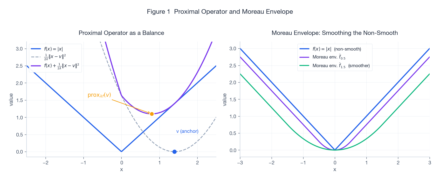
The left panel makes the trade-off visible: blue $f$, grey quadratic anchor, purple sum; the orange dot is $\mathrm{prox}_{\lambda f}(v)$. We will return to the right panel when we reach the Moreau envelope.
Four core properties
These four facts are the bricks for every later analysis.
(1) Existence, uniqueness, and the optimality condition. $\mathrm{prox}_{\lambda f}(v)$ exists and is unique. Moreover, $x^\star = \mathrm{prox}_{\lambda f}(v)$ iff
$$\frac{1}{\lambda}(v - x^\star) \in \partial f(x^\star) \;\;\Longleftrightarrow\;\; v \in x^\star + \lambda\, \partial f(x^\star).$$(2) Fixed-point characterisation. $x^\star$ minimises $f$ iff $x^\star = \mathrm{prox}_{\lambda f}(x^\star)$. This is what lets us turn minimisation into a fixed-point iteration.
(3) Firmly non-expansive. For any $u, v$,
$$\|\mathrm{prox}_{\lambda f}(u) - \mathrm{prox}_{\lambda f}(v)\|_2 \le \|u - v\|_2.$$The stronger “firm” version says $\mathrm{prox}_{\lambda f}$ is a $\tfrac{1}{2}$-averaged map – the main hammer behind ISTA’s convergence.
(4) Separability. If $f(x) = \sum_i f_i(x_i)$, then
$$\bigl[\mathrm{prox}_{\lambda f}(v)\bigr]_i = \mathrm{prox}_{\lambda f_i}(v_i).$$Coordinate-wise functions like $\ell_1$ and box constraints have embarrassingly parallel proxes – this is the reason LASSO scales to millions of features.
Three Workhorse Closed-Form Proxes
L1 norm: the soft-threshold
Let $f(x) = \|x\|_1 = \sum_i |x_i|$. By separability, the problem reduces to one dimension:
$$\min_{x_i} |x_i| + \frac{1}{2\lambda}(x_i - v_i)^2.$$Splitting on the sign of $x_i$ and applying $0 \in \partial(\cdot)$ gives the soft-threshold operator:
$$ \bigl[\mathrm{prox}_{\lambda \|\cdot\|_1}(v)\bigr]_i \;=\; \mathrm{soft}_\lambda(v_i) \;=\; \mathrm{sign}(v_i) \cdot \max\!\bigl(|v_i| - \lambda,\, 0\bigr). $$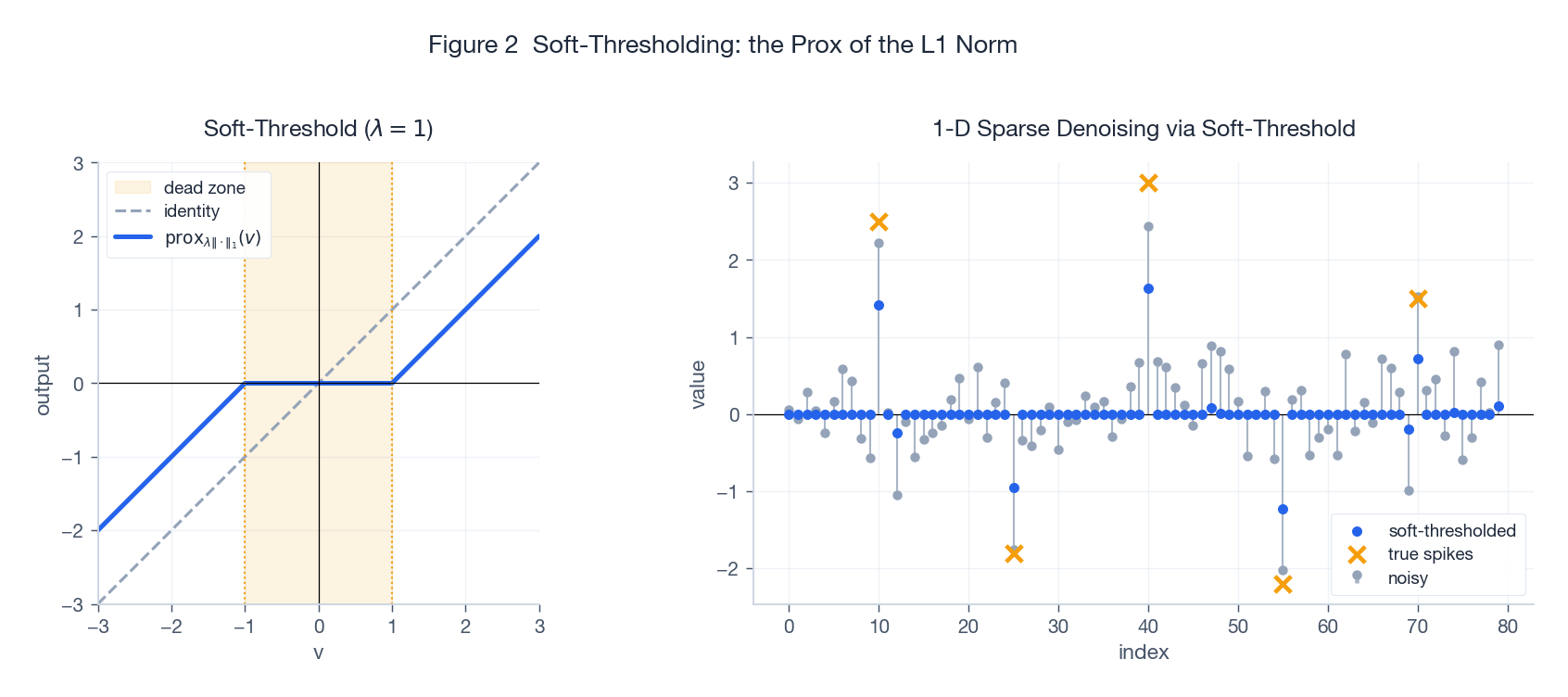
- Left: inside the dead zone $|v| \le \lambda$ the output is exactly zero; outside, $v$ is shrunk toward zero by $\lambda$ (note: shrinkage, not truncation).
- Right: pass a noisy signal through one round of soft-thresholding – small noise is mapped to exact zero, the spikes survive with a mild shrink. This is the mechanism by which LASSO drives unimportant coefficients to exactly zero.
Implementation note: vectorised in one line of NumPy: np.sign(v) * np.maximum(np.abs(v) - lam, 0.0).
Indicator function: the projection
For a convex set $C$, the indicator
$$\iota_C(x) = \begin{cases} 0, & x \in C, \\ +\infty, & x \notin C, \end{cases}$$is convex. Its prox is the Euclidean projection:
$$\mathrm{prox}_{\lambda \iota_C}(v) = \arg\min_{x \in C} \tfrac{1}{2}\|x - v\|_2^2 = P_C(v).$$Note the result is independent of $\lambda$ (the indicator is either $0$ or $+\infty$). This makes “projected gradient descent” a special case of “proximal gradient” – a hard constraint is just an infinitely strong penalty.
Common projections:
- $\ell_2$ ball $\{x : \|x\|_2 \le r\}$: $P(v) = v \cdot \min(1, r / \|v\|_2)$.
- $\ell_\infty$ ball $\{x : \|x\|_\infty \le 1\}$: $P(v)_i = \mathrm{clip}(v_i, -1, 1)$.
- Non-negative orthant $\mathbb{R}^n_{+}$: $P(v) = \max(v, 0)$ (yes, this is ReLU).
- Simplex / $\ell_1$ ball: needs a sort, $O(n \log n)$ but well-known.
Squared norm: linear shrinkage
Let $f(x) = \tfrac{1}{2}\|x\|_2^2$. The first-order condition $x + \tfrac{1}{\lambda}(x - v) = 0$ gives
$$\mathrm{prox}_{\lambda f}(v) = \frac{v}{1 + \lambda}.$$Pure linear shrinkage toward the origin – this is the proximal form of ridge regularisation.
More general quadratic $f(x) = \tfrac{1}{2}x^\top Q x + b^\top x$ ($Q \succeq 0$):
$$\mathrm{prox}_{\lambda f}(v) = (I + \lambda Q)^{-1}(v - \lambda b),$$requiring a single linear solve – still very practical when $Q$ is sparse or structured.
When there is no closed form
Not every $f$ has a closed-form prox. Standard fall-backs:
- Semi-smooth Newton / Newton-CG on the first-order optimality condition.
- Solve the dual – many composite proxes are easier in the dual (see Moreau decomposition below).
- Embed inside ADMM to split a hard prox into two easy ones.
Moreau Envelope: Smoothing the Non-Smooth
Definition and picture
For a closed proper convex $f$ and $\lambda > 0$, the Moreau envelope is
$$\widehat{f}_\lambda(x) \;=\; \min_{y \in \mathbb{R}^n}\left\{ f(y) + \frac{1}{2\lambda}\|y - x\|_2^2 \right\}.$$The envelope is the value (a scalar), the prox is the arg min (a vector). They are born from the same minimisation, hence the tight relation that follows.
Back to Figure 1 right panel: purple and green are the Moreau envelopes of $f(x) = |x|$ at $\lambda = 0.5$ and $\lambda = 1.5$ – this is the Huber function. The kink at zero is rounded into a smooth arc, and the minimum value and the minimiser are preserved.
Three key properties
(1) Same minimum value, same minimiser.
$$\inf_x f(x) = \inf_x \widehat{f}_\lambda(x), \qquad \arg\min f = \arg\min \widehat{f}_\lambda.$$(2) $\widehat{f}_\lambda$ is convex and $\tfrac{1}{\lambda}$-smooth. Even when $f$ is non-differentiable everywhere, $\widehat{f}_\lambda$ is everywhere differentiable with $\tfrac{1}{\lambda}$-Lipschitz gradient.
(3) Gradient identity (the workhorse):
$$\nabla \widehat{f}_\lambda(x) \;=\; \frac{1}{\lambda}\bigl(x - \mathrm{prox}_{\lambda f}(x)\bigr).$$Why this matters: it turns “do gradient descent on the envelope” into “compute one prox” – the algorithmic content of ISTA below.
Short derivation: let $y^\star = \mathrm{prox}_{\lambda f}(x)$. First-order optimality gives $0 \in \partial f(y^\star) + \tfrac{1}{\lambda}(y^\star - x)$, i.e. $\tfrac{1}{\lambda}(x - y^\star) \in \partial f(y^\star)$. Differentiate $\widehat{f}_\lambda(x) = f(y^\star) + \tfrac{1}{2\lambda}\|y^\star - x\|^2$ in $x$ via the envelope theorem – the inner partial in $y$ vanishes by optimality, leaving $\nabla_x \tfrac{1}{2\lambda}\|y - x\|^2 \big|_{y = y^\star} = \tfrac{1}{\lambda}(x - y^\star)$.
Moreau decomposition
A useful duality identity: for a closed proper convex $f$ with conjugate $f^*$,
$$v = \mathrm{prox}_{\lambda f}(v) + \lambda \cdot \mathrm{prox}_{f^* / \lambda}(v / \lambda).$$In practice: if $f$’s prox is hard but $f^*$’s prox is easy (or vice versa), compute on the easy side. The classic application is the nuclear-norm prox (an SVD soft-threshold) versus a spectral-norm projection.
Proximal Gradient: ISTA
Setup
Consider the composite optimisation problem
$$\min_{x \in \mathbb{R}^n} F(x) \;=\; g(x) + h(x),$$where
- $g$ is convex and differentiable with $L$-Lipschitz gradient (the “smooth part”),
- $h$ is convex, possibly non-smooth, but with easy $\mathrm{prox}_{\lambda h}$ (the “non-smooth part”).
LASSO is the prototypical case: $g(x) = \tfrac{1}{2}\|Ax - y\|_2^2$ smooth, $h(x) = \mu \|x\|_1$ via soft-threshold.
ISTA iteration
ISTA (Iterative Shrinkage-Thresholding Algorithm) combines “one gradient step on $g$” with “one prox on $h$”:
$$ \boxed{\;x_{k+1} \;=\; \mathrm{prox}_{\eta h}\!\bigl(x_k - \eta \nabla g(x_k)\bigr).\;} $$Majorisation view: replace $g$ by its quadratic upper bound $\widetilde{g}(x; x_k) = g(x_k) + \langle \nabla g(x_k), x - x_k \rangle + \tfrac{1}{2\eta}\|x - x_k\|_2^2$, then minimise $\widetilde{g}(x; x_k) + h(x)$ – this is exactly the prox above. ISTA is therefore an instance of MM (majorisation-minimisation).
Step-size: $\eta \le 1 / L$ where $L$ is the Lipschitz constant of $\nabla g$. For LASSO, $L = \|A\|_2^2$ (squared largest singular value). Two or three power iterations suffice in practice.
Rate: for convex $F$,
$$F(x_k) - F^\star \le \frac{\|x_0 - x^\star\|_2^2}{2\eta k} = O(1 / k).$$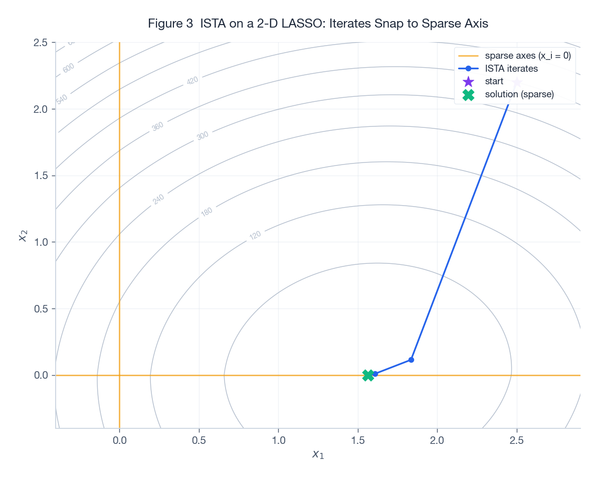
Figure 3 runs ISTA on a 2-D LASSO. The grey contours are the objective; the orange line is the sparse axis ($x_2 = 0$). Starting from the purple star in the upper right, ISTA’s iterates (blue polyline) march toward the optimum and land exactly on $x_2 = 0$ – the sparsity-inducing effect of the soft-threshold made visible.
Acceleration: FISTA
The algorithm
ISTA’s $O(1/k)$ rate is slow on large problems. FISTA (Beck & Teboulle, 2009) borrows Nesterov momentum: take the gradient at an extrapolated point, not at the current iterate.
$$ \begin{aligned} y_k &= x_k + \frac{t_{k-1} - 1}{t_k}\bigl(x_k - x_{k-1}\bigr), \\ x_{k+1} &= \mathrm{prox}_{\eta h}\!\bigl(y_k - \eta \nabla g(y_k)\bigr), \\ t_{k+1} &= \frac{1 + \sqrt{1 + 4 t_k^2}}{2}. \end{aligned} $$Initialise $t_0 = 1$, $x_0 = x_{-1}$.
Rate: $F(x_k) - F^\star \le \dfrac{2 \|x_0 - x^\star\|_2^2}{\eta (k + 1)^2} = O(1/k^2)$.
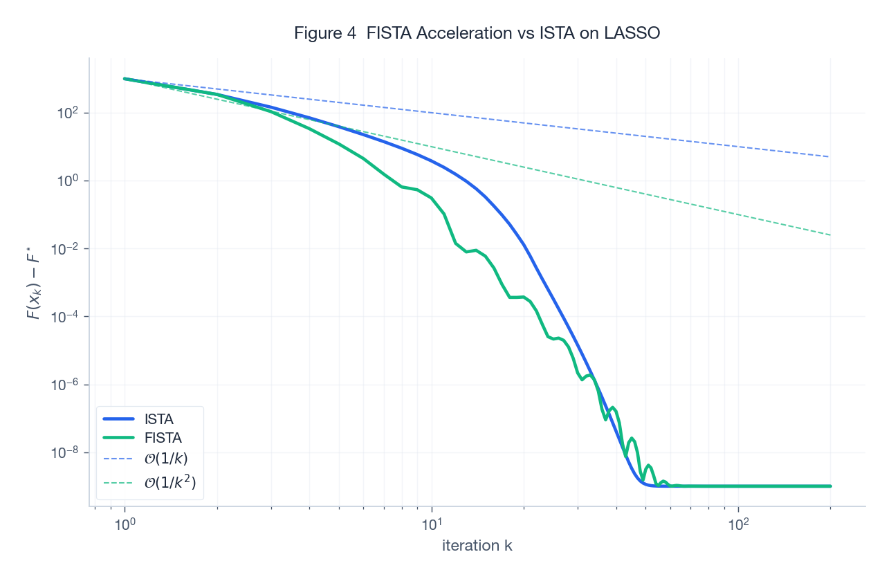
Figure 4 plots the suboptimality gap of ISTA vs FISTA on a 60-D LASSO in log-log. The two reference dashed lines ($1/k$ and $1/k^2$) sit nearly parallel to the empirical curves – the acceleration is real, and within the first 50 iterations FISTA already beats ISTA by roughly an order of magnitude.
Implementation notes
- Restart: $t_k$ is monotone increasing, which can over-extrapolate when the objective oscillates. The cheap fix is function restart: if $F(x_{k+1}) > F(x_k)$, reset $t_k = 1$. In practice this is worth another 2-3x speed-up.
- Strongly convex case: if $g$ is also $\mu$-strongly convex, variants like APGD give linear convergence $(1 - \sqrt{\mu/L})^k$.
- Inexact prox: FISTA still keeps its accelerated rate when the prox is solved approximately, provided the residual decays at $1/k^{3/2}$.
Application: Solving LASSO
Problem and the geometry of the solution
LASSO:
$$\min_x \;\tfrac{1}{2}\|Ax - y\|_2^2 + \mu \|x\|_1.$$The key phenomenon: as $\mu$ increases, more and more coefficients are pushed to exactly zero – this is what makes LASSO simultaneously a fitting and a feature-selection tool.
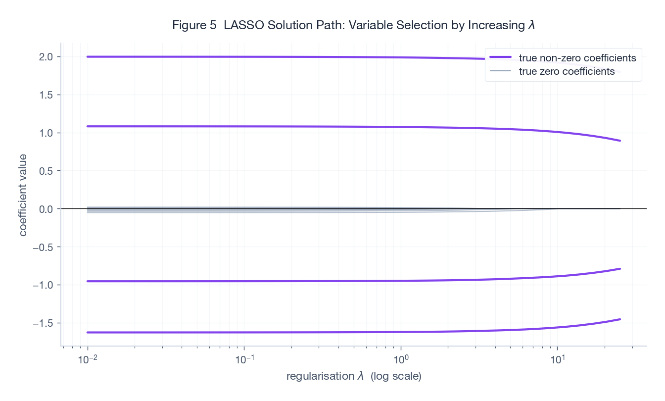
Figure 5 is the classical LASSO path: $\mu$ on the log-scaled x-axis, coefficients on the y-axis. Purple solid = the 4 truly non-zero features, grey dashed = the 8 truly zero features.
- Small $\mu$: every coefficient is non-zero (close to OLS).
- Larger $\mu$: the grey (irrelevant) features are zeroed first; the purple (relevant) features survive longest.
- Picking $\mu$ via cross-validation lands you on a sparse, predictive model.
A clean ISTA / FISTA implementation
| |
Practical notes:
- $L = \|A\|_2^2$ is best estimated by power iteration (avoid a full SVD).
- Use a relative-change check, not gradient norm (the gradient does not exist at kinks).
- For a path of solutions, sweep $\mu$ from large to small with warm starts – huge speed-up.
Subgradient Method vs Proximal Method
The subgradient method is the “raw” tool for non-smooth problems:
$$x_{k+1} = x_k - \eta_k g_k, \quad g_k \in \partial F(x_k),$$but its rate is only $O(1/\sqrt{k})$ and it needs diminishing step-sizes $\eta_k = O(1/\sqrt{k})$ for convergence.
Comparison:
| Method | Structure required | Rate (convex) | Implementation effort | Notes |
|---|---|---|---|---|
| Subgradient | any convex $F$ | $O(1/\sqrt{k})$ | low | universal but slow |
| ISTA | $g$ smooth + $h$ easy prox | $O(1/k)$ | low | the LASSO default |
| FISTA | same as ISTA | $O(1/k^2)$ | medium | go-to for large scale |
| ADMM | $\min g(x) + h(z)$ s.t. $Ax + Bz = c$ | $O(1/k)$ (general convex) | medium | splittable composites |
Practical advice: prefer proximal methods whenever the non-smooth piece can be split out and admits a tractable prox – you typically gain orders of magnitude in real problems.
ADMM in One Page
When the problem has two non-smooth terms or linear equality constraints, ISTA / FISTA alone is not enough. ADMM (Alternating Direction Method of Multipliers) writes the problem as
$$\min_{x, z}\; g(x) + h(z) \quad \text{s.t.}\quad Ax + Bz = c,$$and alternates:
$$ \begin{aligned} x_{k+1} &= \arg\min_x\; g(x) + \tfrac{\rho}{2}\|Ax + Bz_k - c + u_k\|_2^2, \\ z_{k+1} &= \arg\min_z\; h(z) + \tfrac{\rho}{2}\|Ax_{k+1} + Bz - c + u_k\|_2^2, \\ u_{k+1} &= u_k + Ax_{k+1} + Bz_{k+1} - c. \end{aligned} $$Each subproblem now contains only one non-smooth term, so each can be solved by a single prox.
LASSO via ADMM: rewrite the constraint as $x = z$. The $x$-update is the closed-form ridge solution; the $z$-update is the soft-threshold. Clean.
ADMM’s strengths:
- Two non-smooth terms summed (e.g. $\ell_1$ + total variation).
- Naturally distributed (consensus ADMM).
- $O(1/k)$ for general convex; constants are often smaller than ISTA in practice.
ADMM’s costs: pick $\rho$, solve a linear system in the $x$-update.
Convergence: Practical Side
What to monitor in ISTA / FISTA
- Monotone decrease of the objective (ISTA) / strict decrease after restarts (FISTA).
- $\|x_{k+1} - x_k\|$ down to a tolerance – the most reliable check in the non-smooth setting.
- Stability of the active set: once the support of $x_k$ stops changing, you are essentially at the optimum.
Common traps
- Step-size too large: $\eta > 1/L$ diverges. If $L$ is uncertain, use backtracking line search: try $\eta \cdot \beta$ each iteration, halve when the sufficient-decrease condition fails.
- Cold-starting every $\mu$ on a path: enormous waste – always warm-start.
- Conflating $\lambda$ and $\eta$: the threshold inside $\mathrm{prox}_{\eta \cdot \mu \|\cdot\|_1}$ is $\eta \mu$, not $\mu$ and not $\eta$.
- Plain gradient descent on hinge / $\ell_1$: chatters around the kinks. Use a prox or a subgradient.
Exercises
Exercise 1: closed-form proxes
Compute $\mathrm{prox}_{\lambda f}$ for each:
(a) $f(x) = \|x\|_1$.
Solution: by separability + 1-D subgradient analysis,
$$\bigl[\mathrm{prox}_{\lambda f}(v)\bigr]_i = \mathrm{sign}(v_i)\max(|v_i| - \lambda, 0).$$(b) $f(x) = \iota_{B_\infty}(x)$ where $B_\infty = \{x : \|x\|_\infty \le 1\}$.
Solution: project to the $\ell_\infty$ ball, coordinate-wise clip:
$$\bigl[\mathrm{prox}_{\lambda f}(v)\bigr]_i = \min\bigl(\max(v_i, -1),\, 1\bigr).$$Note the result is independent of $\lambda$.
(c) $f(x) = \tfrac{\beta}{3}\|x\|_3^3$ ($\beta > 0$).
Solution: separable. For $v_i \ge 0$ the minimiser $x_i \ge 0$ solves $\beta x_i^2 + \tfrac{1}{\lambda}(x_i - v_i) = 0$, i.e. $\lambda \beta x_i^2 + x_i - v_i = 0$:
$$\bigl[\mathrm{prox}_{\lambda f}(v)\bigr]_i = \mathrm{sign}(v_i) \cdot \frac{-1 + \sqrt{1 + 4\lambda\beta |v_i|}}{2\lambda\beta}.$$A rare case where an $\ell_p$ norm with $p > 2$ has a closed-form prox.
Exercise 2: differentiability of the Moreau envelope
Show that the Moreau envelope $\widehat{f}_\lambda$ of a closed proper convex $f$ is differentiable everywhere with
$$\nabla \widehat{f}_\lambda(x) = \frac{1}{\lambda}\bigl(x - \mathrm{prox}_{\lambda f}(x)\bigr).$$Sketch:
- The minimiser is unique, so $y(x) := \mathrm{prox}_{\lambda f}(x)$ is single-valued. By non-expansiveness, $y(x)$ is 1-Lipschitz in $x$.
- The first-order condition gives $\tfrac{1}{\lambda}(x - y(x)) \in \partial f(y(x))$.
- Apply the envelope theorem to $\widehat{f}_\lambda(x) = f(y(x)) + \tfrac{1}{2\lambda}\|y(x) - x\|^2$. The inner partial in $y$ vanishes by optimality, leaving $\nabla_x \tfrac{1}{2\lambda}\|y - x\|^2 \big|_{y = y(x)} = \tfrac{1}{\lambda}(x - y(x))$.
Since $y(x)$ is 1-Lipschitz, $\nabla \widehat{f}_\lambda$ is $\tfrac{1}{\lambda}$-Lipschitz – hence the envelope is automatically 1-smooth.
Exercise 3: why the SVM prox is “useless”
Take a linear SVM $f(w) = \sum_i \max(0, 1 - y_i x_i^\top w) + \tfrac{\lambda}{2}\|w\|_2^2$.
(a) Give a subgradient of $f$ at $w$.
Solution: for hinge $\ell_i(w) = \max(0, 1 - y_i x_i^\top w)$,
$$ \partial \ell_i(w) = \begin{cases} \{0\}, & y_i x_i^\top w > 1, \\ \{- y_i x_i\}, & y_i x_i^\top w < 1, \\ [-y_i x_i, 0], & y_i x_i^\top w = 1. \end{cases} $$Total: $\partial f(w) \ni \sum_i g_i + \lambda w$ for any $g_i \in \partial \ell_i(w)$.
(b) Show that computing $\mathrm{prox}_{\alpha f}(0)$ is essentially as hard as solving the SVM itself.
Solution: by definition,
$$\mathrm{prox}_{\alpha f}(0) = \arg\min_w \;\sum_i \max(0, 1 - y_i x_i^\top w) + \tfrac{1}{2}\!\left(\lambda + \tfrac{1}{\alpha}\right)\|w\|_2^2.$$This is itself an SVM, just with regularisation strength $\lambda + 1/\alpha$ instead of $\lambda$. The takeaway: don’t try to compute the prox of an entire complicated objective – proximal methods only buy you something when there is a non-smooth piece that can be cleanly split out.
Exercise 4: projected gradient is a special case of ISTA
Show that constrained optimisation $\min_{x \in C} g(x)$ ($g$ smooth, $C$ closed convex) is equivalent to the composite $\min_x g(x) + \iota_C(x)$, and write down the ISTA iteration.
Solution: with $h = \iota_C$, $\mathrm{prox}_{\eta h}(v) = P_C(v)$. Plug into ISTA:
$$x_{k+1} = P_C\!\bigl(x_k - \eta \nabla g(x_k)\bigr).$$This is exactly projected gradient descent – ISTA with $h = \iota_C$. Adding momentum gives accelerated projected gradient.
Summary
The point of the proximal operator is concrete: isolate “non-smooth” or “constrained” out of the main problem and turn it into a small subproblem. Concretely:
- Lebesgue non-differentiability of $\ell_1$ -> soft-threshold.
- A convex constraint -> projection.
- The whole non-smooth function -> a Moreau envelope you can differentiate.
The minimum operational checklist:
- ISTA: $x_{k+1} = \mathrm{prox}_{\eta h}(x_k - \eta \nabla g(x_k))$, $\eta \le 1/L$, $O(1/k)$.
- FISTA: ISTA step at the extrapolation point, update $t_k$; $O(1/k^2)$, function-restart in practice.
- LASSO: FISTA + soft-threshold + warm-start across $\mu$ – the industry default for $\ell_1$.
- ADMM: when there are two non-smooth pieces or equality constraints, split by variable and alternate.
Keep these tools at hand. Next time $\|\cdot\|_1$, $\iota_C$, total variation, or a nuclear norm shows up in your objective, none of it will feel scary – it is all just one prox away.
Further reading
- N. Parikh, S. Boyd. Proximal Algorithms. Foundations and Trends in Optimization, 2014. (The canonical survey.)
- A. Beck, M. Teboulle. A Fast Iterative Shrinkage-Thresholding Algorithm for Linear Inverse Problems. SIAM J. Imaging Sciences, 2009. (FISTA original paper.)
- S. Boyd et al. Distributed Optimization and Statistical Learning via the Alternating Direction Method of Multipliers. FnTML, 2011. (ADMM survey.)
- L. Condat et al. Proximal Splitting Algorithms for Convex Optimization: A Tour of Recent Advances. SIAM Review, 2023. (Latest survey including PDHG / Condat-Vu.)