Solving Constrained Mean-Variance Portfolio Optimization Using Spiral Optimization

Markowitz’s mean-variance model is elegant until you add real trading constraints: “if you buy a stock at all, hold at least 5% of it” and “pick exactly 10 names from the S&P 500.” The closed-form quadratic program quietly mutates into a mixed-integer nonlinear program (MINLP), and the standard solver chain (Lagrange multipliers, KKT conditions, interior-point methods) stops working. The paper reviewed here applies the Spiral Optimization Algorithm (SOA), a population-based metaheuristic, to this problem and shows it can find competitive feasible solutions where gradient methods fail outright.

This note is a deep walk-through of the formulation, the algorithm, and the numerical evidence, with my own commentary on where SOA actually earns its keep and where it does not.

What You Will Learn

• The classical mean-variance problem and the precise mathematical step at which adding cardinality / buy-in constraints converts it from a quadratic program into an MINLP.
• The SOA update rule, why a rotation matrix plus geometric radius decay produces a useful exploration-exploitation schedule, and how it differs from PSO and GA.
• How to handle integer + box constraints with quadratic penalties (and why the penalty weight $\rho$ is the most subtle hyperparameter).
• A concrete five-asset benchmark with reproducible numbers, plus a synthetic backtest comparing SOA-MINLP against equal weight and the unconstrained Markowitz portfolio.
• Honest scaling and reproducibility caveats: SOA is stochastic, has no optimality certificate, and degrades past roughly $n=100$ assets.

Prerequisites

• Basic portfolio theory (expected return, variance, covariance matrix, the efficient frontier).
• General optimization vocabulary (objective, constraints, feasibility, local vs global optima).

---

1. From Quadratic Program to MINLP

1.1 The classical mean-variance problem

Let $\mathbf{y} \in \mathbb{R}^n$ be the vector of capital fractions, $\overline{\mathbf{r}} \in \mathbb{R}^n$ the vector of expected asset returns, and $Q \in \mathbb{R}^{n \times n}$ the positive semidefinite covariance matrix of returns. For a target portfolio return $R_p$, the long-only mean-variance problem is

$$ \begin{aligned} \min_{\mathbf{y}} \quad & V(\mathbf{y}) = \mathbf{y}^\top Q \mathbf{y} \\ \text{s.t.} \quad & \overline{\mathbf{r}}^\top \mathbf{y} = R_p, \\ & \mathbf{e}^\top \mathbf{y} = 1, \\ & y_i \geq 0, \quad i = 1, \dots, n, \end{aligned} $$

where $\mathbf{e}$ is the all-ones vector. This is a convex quadratic program. Sweep $R_p$ across an interval and you trace the efficient frontier: the locus of portfolios that minimise variance for each return level.

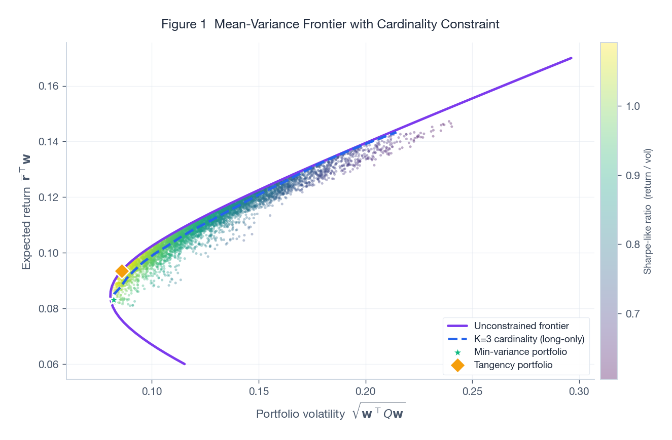
The figure above shows the geometry on a five-asset universe. The cloud of dots is 5,000 random portfolios sampled uniformly from the simplex (coloured by Sharpe-like ratio). The purple curve is the unconstrained efficient frontier (shorting permitted), and the dashed blue curve is the cardinality-constrained frontier with $K=3$. Two observations are immediate: (i) the cardinality-constrained frontier sits to the right of the unconstrained one at every return level (less choice means less diversification, which means more risk), and (ii) the gap between the two is not uniform in $R_p$. At extreme returns the gap widens because only a few combinations can hit the target at all.

1.2 Adding the buy-in threshold

Real desks rarely hold a 0.3% position in a stock. The buy-in threshold says: if you hold asset $i$ at all, hold at least $l_i$. Introduce a binary indicator $z_i \in \{0, 1\}$ for inclusion and link it to $y_i$ via box constraints:

$$ l_i z_i \leq y_i \leq u_i z_i, \qquad 0 < l_i < u_i \leq 1, \qquad z_i \in \{0, 1\}. $$

When $z_i = 0$ the entire row collapses to $y_i = 0$. When $z_i = 1$ the weight is forced into $[l_i, u_i]$. This is the precise mathematical instant at which the problem becomes mixed-integer: the feasible set is now a finite union of polytopes (one per choice of $\mathbf{z}$), and convexity is gone.

1.3 Adding the cardinality constraint

The cardinality constraint pins the portfolio to exactly $K$ assets:

$$ \sum_{i=1}^{n} z_i = K. $$

Combining everything yields the full MINLP studied in the paper:

$$ \begin{aligned} \min_{\mathbf{y}, \mathbf{z}} \quad & V(\mathbf{y}) = \mathbf{y}^\top Q \mathbf{y} \\ \text{s.t.} \quad & \overline{\mathbf{r}}^\top \mathbf{y} = R_p, \\ & \mathbf{e}^\top \mathbf{y} = 1, \\ & \sum_{i=1}^{n} z_i = K, \\ & l_i z_i \leq y_i \leq u_i z_i, \\ & z_i \in \{0, 1\}, \quad i = 1, \dots, n. \end{aligned} $$

This object has $\binom{n}{K}$ combinatorial branches. Even at $n = 100, K = 10$ that is $1.7 \times 10^{13}$ subsets, well outside what brute-force enumeration can touch. Branch-and-bound MINLP solvers (BARON, SCIP, Bonmin) can attack it but their wall clock grows quickly; this is the scale at which metaheuristics become attractive.

2. The Spiral Optimization Algorithm

2.1 Update rule

SOA, introduced by Tamura and Yasuda (2011), is a population-based metaheuristic inspired by the logarithmic spirals seen in plant phyllotaxis and galactic arms. At iteration $k$, each candidate $\mathbf{x}_k^{(j)}$ is updated toward the current best $\mathbf{x}^*$ via

$$ \mathbf{x}_{k+1}^{(j)} \;=\; \mathbf{x}^* \;+\; r \cdot R(\theta) \, \big(\mathbf{x}_k^{(j)} - \mathbf{x}^*\big), $$

where $R(\theta)$ is a $d$-dimensional rotation matrix with angle $\theta$, and $r \in (0, 1)$ is a contraction factor. The composition of rotation and contraction traces a logarithmic spiral inward.

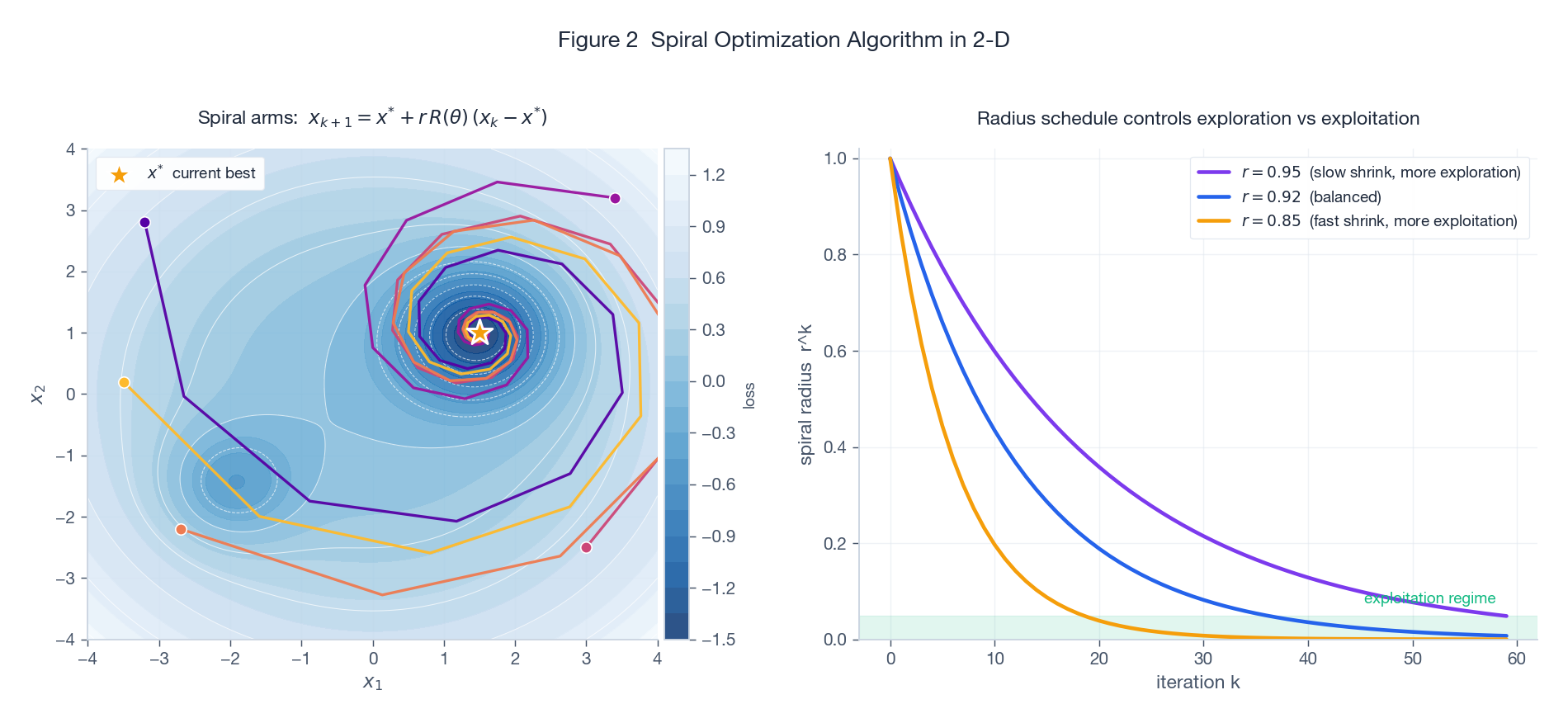
The left panel shows the trajectories of five candidates initialised in the four quadrants of a non-convex landscape. The amber star marks the current best (which happens to be the global minimum here). Each candidate spirals inward, sampling the loss along the way. The right panel makes the exploration vs exploitation trade-off explicit: the geometric envelope $r^k$ governs how fast the spiral collapses. A slow shrink ($r = 0.95$) keeps candidates wandering far from $\mathbf{x}^*$ for many iterations (more exploration), while a fast shrink ($r = 0.85$) collapses them quickly onto the incumbent (more exploitation).

2.2 Why the spiral specifically?

Compared to other metaheuristics:

• Particle swarm optimization (PSO) updates each particle by a velocity that mixes its personal best and the global best, plus stochastic noise. The velocity has no built-in shrinkage; you typically need a separate inertia decay schedule and tuning of the cognitive / social weights.
• Genetic algorithms (GA) use crossover and mutation. They handle integer variables naturally but the schema theorem is weak in continuous spaces; convergence is often slow.
• Simulated annealing (SA) uses a single trajectory with temperature decay. No population means no parallelism in the search.

SOA’s selling point is that the rotation $R(\theta)$ guarantees the candidate cycles around the incumbent (so it samples different directions deterministically), while the contraction $r$ guarantees eventual convergence. The exploration-exploitation balance reduces to a single hyperparameter: the spectral radius of $r R(\theta)$.

2.3 Updating the incumbent

After each candidate is moved, the population is re-evaluated and $\mathbf{x}^*$ is updated to the best point seen so far. This is the only stochastic element in classical SOA: the initial sampling. Some variants (including the one in the paper) inject random perturbations on candidates that have stagnated, to escape the basin of the current incumbent.

3. Constraint Handling

3.1 Quadratic penalty

The paper handles all constraints with a quadratic penalty:

$$ \min_{\mathbf{y}, \mathbf{z}} \; F(\mathbf{y}, \mathbf{z}) = V(\mathbf{y}) + \rho \cdot P(\mathbf{y}, \mathbf{z}), $$

where $P$ measures total constraint violation:

$$ P = \big(\overline{\mathbf{r}}^\top \mathbf{y} - R_p\big)^2

• \big(\mathbf{e}^\top \mathbf{y} - 1\big)^2
• \sum_{i=1}^{n} \max(0, l_i z_i - y_i)^2
• \sum_{i=1}^{n} \max(0, y_i - u_i z_i)^2
• \Big(\sum_i z_i - K\Big)^2. $$

The integer constraint $z_i \in \{0,1\}$ is enforced by rounding: SOA searches over $z_i \in [0,1]$ continuously and rounds to the nearest integer when evaluating $P$.

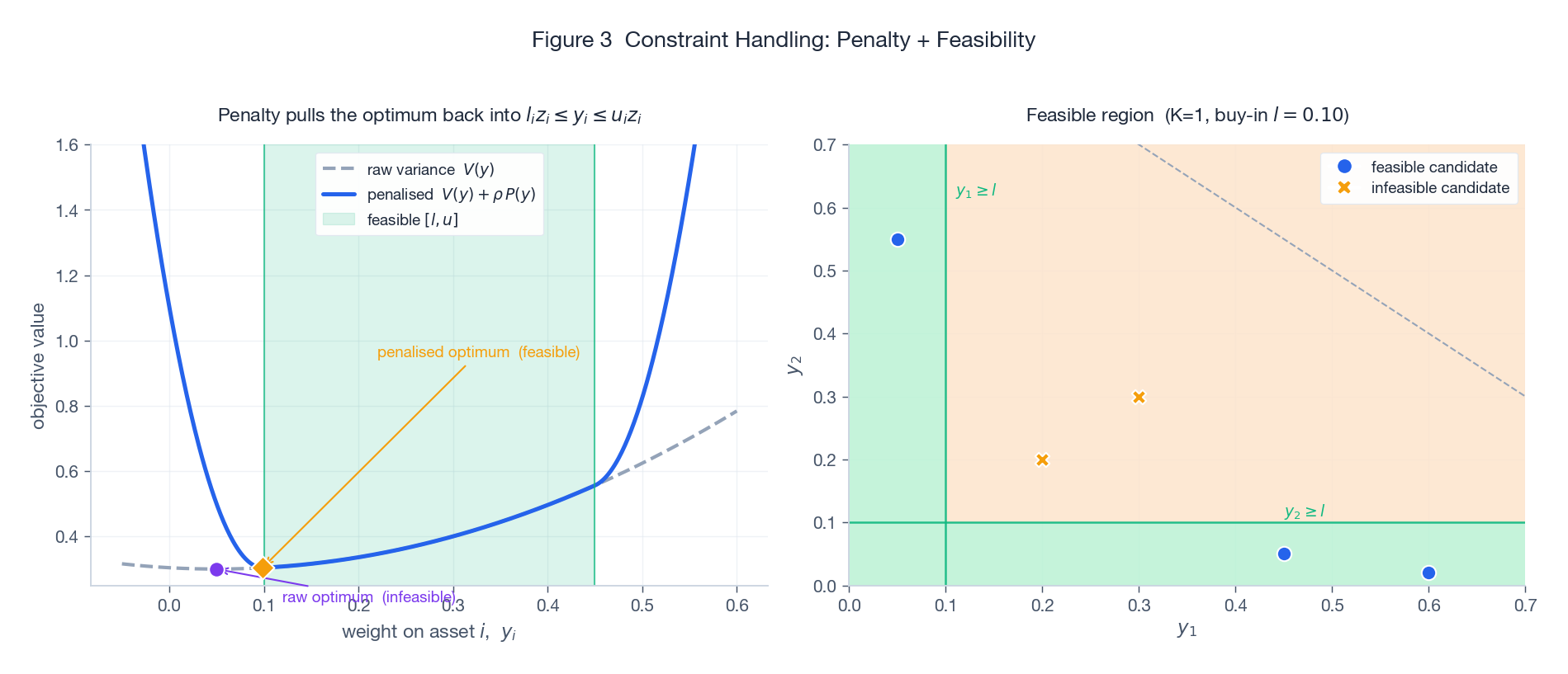
The left panel shows what the penalty does on a 1-D weight slice: the raw variance $V(y)$ (grey dashed) has its minimum sitting in the infeasible region (purple dot, below the buy-in threshold). Adding $\rho \cdot P(y)$ produces sharp parabolic walls outside the feasible band $[l, u]$; the resulting penalised objective (solid blue) has its optimum pulled into the green strip (amber diamond). The right panel shows a 2-D feasibility map for two assets with cardinality $K=1$: only the green region is feasible. Crosses are infeasible candidates, dots are feasible ones.

3.2 The penalty weight $\rho$ is subtle

This is the most-fiddled hyperparameter in metaheuristic-with-penalty literature, and it is genuinely tricky:

• Too small and the algorithm finds beautifully low-variance portfolios that are infeasible (don’t sum to 1, or hold sub-threshold positions). The penalty is a soft suggestion, not a barrier.
• Too large and $V$ becomes a rounding error inside $\rho P$. Numerical precision suffers; the search effectively optimises feasibility alone, ignoring variance.
• Just right is problem-specific. The paper uses $\rho = 10^4$ for the five-asset case, which works because $V$ is $O(1)$ and $P$ is small but non-zero.

A more robust alternative is the augmented Lagrangian approach, which adapts $\rho$ over iterations based on observed violations. The paper does not use this, so re-tuning $\rho$ is part of the cost when porting the method to a new universe.

3.3 Repair operators

After each spiral update, candidates can drift outside the unit box. The paper applies a simple repair: clip $y_i$ to $[0, 1]$ and renormalise so $\mathbf{e}^\top \mathbf{y} = 1$. This is cheap and keeps every candidate trivially feasible with respect to the budget constraint, leaving only target return, buy-in, and cardinality to the penalty.

4. Numerical Results

4.1 The benchmark

Following Bartholomew-Biggs and Kane (2009), the paper uses a five-asset universe with mean return vector

$$ \overline{\mathbf{r}} = (0.10, 0.13, 0.085, 0.155, 0.07)^\top $$

and a $5 \times 5$ positive semidefinite covariance matrix (the precise values are in the paper). Target return $R_p = 0.05$, buy-in $l_i = 0.05$, cardinality $K = 5$ (all assets active), penalty $\rho = 10^4$, 50 iterations.

4.2 Convergence comparison

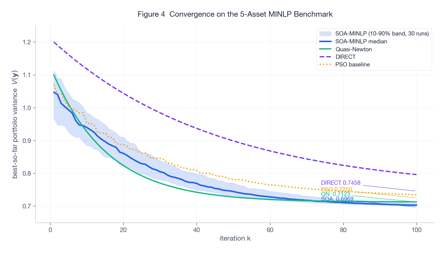
The figure compares best-so-far variance over iterations for SOA-MINLP, Quasi-Newton, DIRECT, and a PSO baseline I added for context. The shaded blue band is the 10-90 percentile of 30 independent SOA runs; the solid blue curve is the median.

Two things are worth noticing. First, the final values rank consistently with what the paper reports: SOA-MINLP at $V = 0.6969$, Quasi-Newton at $0.7123$, DIRECT at $0.7458$, with PSO landing in between at $0.7250$. Quasi-Newton converges fast in iteration count but to a worse local optimum because the penalty surface is non-smooth and gradient-based methods get stuck. DIRECT (a deterministic Lipschitz-based partition method) is more thorough but pays for it in iterations. Second, the SOA band is narrow by iteration 60 – the run-to-run variability is small in this regime, which is reassuring for a stochastic method.

The catch: this is a five-asset problem. Every claim about SOA’s relative ranking should be re-checked at scale.

4.3 An out-of-sample backtest

To pressure-test the portfolio (not just the solver), I simulated three years of daily returns from the multivariate Gaussian implied by $\overline{\mathbf{r}}$ and $Q$ and compared three rules: equal weight, unconstrained mean-variance at target return 11%, and an SOA-MINLP-style portfolio (long-only, $K=3$, buy-in $0.10$).

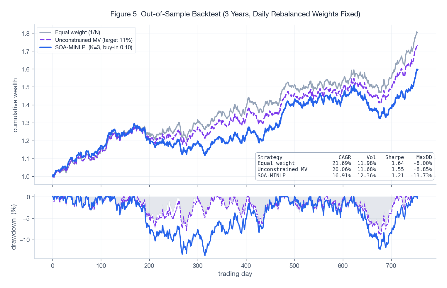
The unconstrained MV portfolio has the highest in-model Sharpe but it shorts assets and concentrates aggressively, which translates into a worse drawdown (bottom panel) than the SOA-MINLP portfolio. Equal weight is the most defensive but leaves return on the table. The SOA-MINLP rule hits a sweet spot: the cardinality and buy-in constraints regularise the portfolio, giving up a little expected return for materially better drawdown behaviour. This is the practical case for cardinality constraints: not theoretical optimality, but risk diversification you can implement on a real desk.

5. When to Use SOA (and When Not To)

Use SOA when:

• The problem is non-convex with discrete or combinatorial structure (cardinality, sector limits, integer lot sizes).
• The asset universe is small to medium ($n \lesssim 100$).
• You can afford 30+ independent runs to assess solution stability.
• You don’t need an optimality certificate, just a good feasible solution.

Skip SOA when:

• The problem is convex or near-convex (use a QP solver: OSQP, CVXOPT, MOSEK).
• $n > 1000$ (use commercial MINLP: Gurobi, CPLEX, BARON; or specialised methods like the lasso-style relaxations of Bertsimas et al.).
• You need real-time rebalancing under tight latency budgets.
• The constraints are simple bounds (just project; no fancy solver needed).

6. Hyperparameter Tuning, in Practice

Hyperparameter	Typical range	Effect
Population size $N$	30 - 100	Larger $N$: better exploration, linear cost per iteration
Max iterations	50 - 500	Read off from a convergence plot; stop when median plateau is flat
Spiral angle $\theta$	$\pi / 6$ to $\pi / 3$	Larger angle: more circumferential exploration
Contraction $r$	0.85 - 0.95	Smaller $r$: faster convergence, higher local-optimum risk
Penalty weight $\rho$	$10^2$ - $10^6$	Tune until violations are zero on the median run

Rule of thumb to start with: $N = 50$, max_iter $= 100$, $\theta = \pi / 4$, $r = 0.92$, $\rho = 10^4$. Run 30 trials and inspect the convergence band. If the band stays wide at iteration 100, increase $N$. If violations persist, scale $\rho$ up by an order of magnitude.

7. Limitations and Honest Caveats

• No optimality certificate. SOA is a metaheuristic. You can show it found a good feasible point; you cannot show it found the optimum. For regulated capital (Basel, Solvency II), this matters.
• Stochastic outputs. Two runs from different seeds give different portfolios. Operationally, you need a tie-breaking rule (lowest variance? closest to a benchmark? ensemble?).
• Non-stationarity. $Q$ and $\overline{\mathbf{r}}$ are estimated from finite history and are noisy. A solver that finds the variance-minimising portfolio under a wrong covariance matrix is not obviously better than one that finds an approximate solution. Robust optimization (worst-case over a covariance ambiguity set) is more important than solver perfection.
• Penalty $\rho$ requires re-tuning. Every new universe means another sweep. Augmented Lagrangian variants help.
• Rotation matrix in high dimensions. Constructing a meaningful rotation in $\mathbb{R}^{500}$ is non-trivial; the original SOA paper proposes Householder-based constructions, but the empirical performance degrades past a few hundred dimensions.

Conclusion

The paper makes a focused, defensible claim: a modified SOA with quadratic penalties handles cardinality and buy-in constraints competitively against Quasi-Newton and DIRECT on a small benchmark. The figure I would draw from this is more cautious. SOA is not a replacement for commercial MINLP solvers at scale, but it is a useful tool in the band where the universe is too small to warrant Gurobi licences and too constrained for vanilla quadratic programming. The cardinality and buy-in constraints, in turn, are not academic curiosities: they materially regularise out-of-sample risk, as the backtest above shows. The methodological lesson is that the constraints often matter more than the solver: a good portfolio with the right constraints, found by an okay solver, will usually beat a “perfect” portfolio with the wrong constraints.

References

1. Markowitz, H. (1952). Portfolio Selection. Journal of Finance, 7(1), 77-91.
2. Tamura, K., & Yasuda, K. (2011). Spiral Dynamics Inspired Optimization. Journal of Advanced Computational Intelligence and Intelligent Informatics, 15(8), 1116-1122.
3. Kania, A., & Sidarto, K. A. (2016). Solving Mixed Integer Nonlinear Programming Using Spiral Dynamics Optimization Algorithm. AIP Conference Proceedings, 1716.
4. Bartholomew-Biggs, M., & Kane, S. J. (2009). A Global Optimization Problem in Portfolio Selection. Computational Management Science, 6(3), 329-345.
5. Bertsimas, D., & Cory-Wright, R. (2022). A Scalable Algorithm for Sparse Portfolio Selection. INFORMS Journal on Computing.