A plain autoencoder compresses and reconstructs. A variational autoencoder learns something far more useful: a smooth, structured latent space you can sample from to generate genuinely new data. That single change — making the encoder output a distribution instead of a vector — turns the network from a fancy compressor into a generative model with a tractable likelihood lower bound.

This guide walks the full path: why autoencoders fail at generation, how the ELBO derivation gets you to the loss function, why the reparameterization trick is the trick that makes everything trainable, a complete PyTorch implementation, and a tour of every common failure mode with concrete fixes.

What you will learn

• Why an autoencoder’s latent space is unusable for sampling, and what VAEs change
• The ELBO objective: how reconstruction and KL fall out of a single likelihood bound
• The reparameterization trick: why naive sampling breaks gradients, and how mu + sigma * eps fixes it
• A complete PyTorch implementation: encoder, decoder, loss, training loop, sampling, interpolation
• Failure modes you will hit: posterior collapse, blurry samples, NaN gradients — with diagnostic and fix
• Useful variants: beta-VAE, conditional VAE, hierarchical VAE
• When to reach for a VAE versus a GAN or diffusion model

Prerequisites

• PyTorch basics (nn.Module, forward/backward, optimizers)
• Probability foundations (mean, variance, the Gaussian density)
• Some experience training neural networks end-to-end

Why VAEs matter: autoencoders versus generative models

The autoencoder baseline

An autoencoder pairs an encoder $f_\phi$ with a decoder $g_\theta$. It learns to compress input $x$ into a code $z = f_\phi(x)$ and then reconstruct $\hat{x} = g_\theta(z)$. The training objective is just reconstruction error:

This works fine for compression and denoising, but it gives you a latent space that is deterministic and unstructured. Concretely:

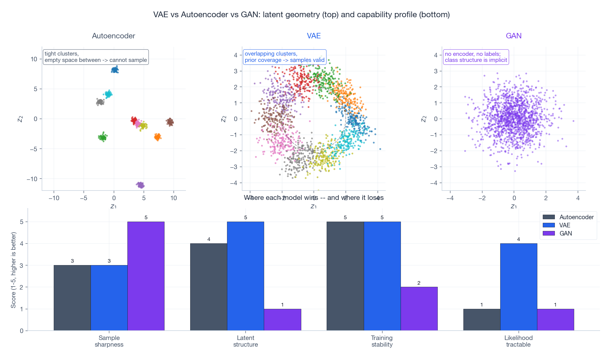
• You cannot sample. The decoder has only ever seen codes that the encoder produced. A random $z$ drawn from anywhere in the space will likely fall in a hole the decoder never visited and produce garbage.
• Interpolation is brittle. Two visually similar inputs can land at distant points; two distant inputs can land near each other. A straight line in latent space passes through nonsense.
• There is no probabilistic interpretation. No prior, no likelihood, no way to talk about how likely a generated sample is.

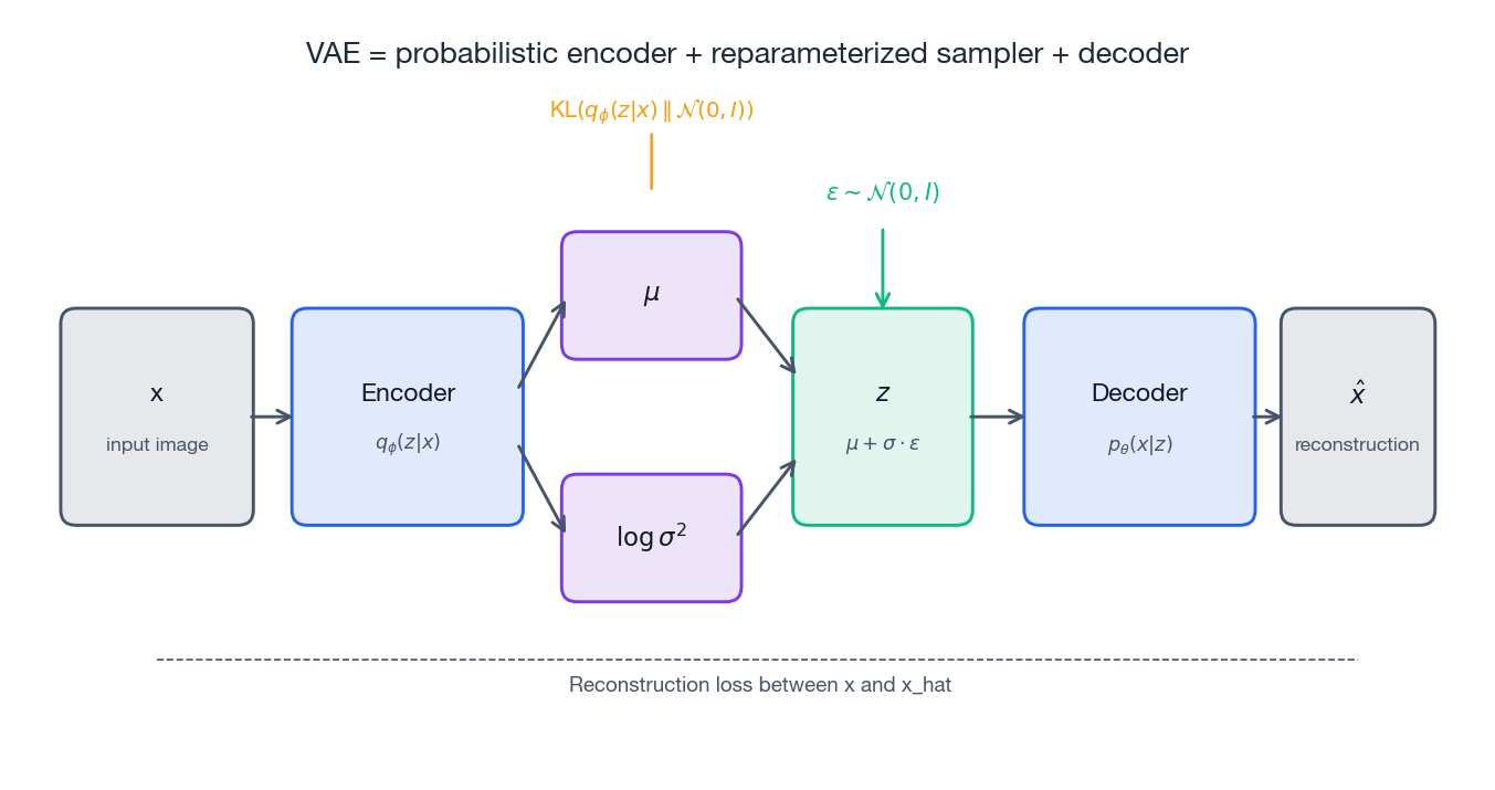
What VAEs change: a probabilistic latent

A VAE replaces the deterministic encoding with a distribution. The encoder outputs the parameters of a Gaussian:

The decoder defines a likelihood $p_\theta(x \mid z)$, and we impose a fixed prior $p(z) = \mathcal{N}(0, I)$.

Three benefits flow from this single change:

1. Sampling works. Draw $z \sim p(z)$, feed it to the decoder, get a fresh $\hat{x}$.
2. Interpolation is smooth. Encoder distributions for similar inputs overlap, so straight lines through latent space yield gradual morphs.
3. Structure is enforced. The KL term in the loss (next section) actively pushes the aggregated posterior toward the prior, filling the space evenly.

The ELBO objective: where the loss comes from

Deriving the bound

We want to maximize the data log-likelihood $\log p_\theta(x)$, but it involves an intractable integral over $z$. The trick is to introduce the variational posterior $q_\phi(z \mid x)$ and apply Jensen’s inequality:

This right-hand side is the Evidence Lower BOund (ELBO). Maximizing it does two things at once:

• Reconstruction term $\mathbb{E}_{q_\phi}[\log p_\theta(x \mid z)]$: the decoder must explain $x$ well from a code sampled by the encoder.
• KL term $D_{\mathrm{KL}}(q_\phi(z\mid x)\,\|\,p(z))$: the encoder cannot wander wherever it likes; it must stay close to the prior.

In code, we minimize the negative ELBO. With a Gaussian encoder and a standard normal prior, the KL term has a closed form per dimension:

Why the KL term is load-bearing

Without KL regularization, two pathologies appear immediately:

• Spike-and-gap latent. The encoder collapses each $x$ onto an isolated point with tiny variance. The space is a constellation of needles in vacuum — beautiful for reconstruction, useless for generation.
• Decoder ignores $z$. With a powerful decoder you also see the opposite extreme (called posterior collapse, discussed below).

The KL term forces $q_\phi(z\mid x)$ for different inputs to overlap and to cover the prior. That overlap is what makes interpolation smooth and what makes the prior usable as a sampler.

The reparameterization trick

The problem: gradients can’t pass through a sample

To estimate the reconstruction term we need to draw $z \sim q_\phi(z \mid x)$ and run the decoder. But sampling is a stochastic node — backpropagation cannot pass a gradient through “draw a random number.” If we naively sample, $\nabla_\phi$ for the encoder is undefined.

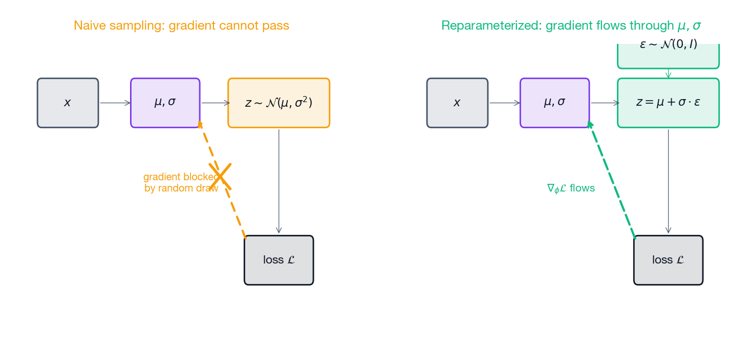
The fix: move randomness outside the parameter path

Rewrite the sample as a deterministic function of the parameters and an external noise source:

Now $\epsilon$ has no parameters, and the path from $\phi$ to $z$ is fully differentiable. Gradients flow cleanly through $\mu$ and $\sigma$.

 1
 2
 3
 4
 5
 6
 7
 8
 9
10
11
12

def reparameterize(mu, logvar):
    """Sample z ~ N(mu, sigma^2) in a differentiable way.

    Args:
        mu:     (B, latent_dim) encoder mean
        logvar: (B, latent_dim) encoder log-variance
    Returns:
        z:      (B, latent_dim) sample
    """
    std = torch.exp(0.5 * logvar)
    eps = torch.randn_like(std)
    return mu + std * eps

Why predict logvar instead of sigma? Two reasons, both about numerical safety:

• logvar is unconstrained — any real number is valid. Predicting sigma directly forces you to enforce $\sigma > 0$ (e.g., softplus), which is one more thing to get wrong.
• The closed-form KL involves $\log \sigma^2$. Predicting it directly avoids log(exp(...)) round-trips that can underflow.

Complete PyTorch implementation

The model below is the canonical “MNIST VAE”: fully connected encoder/decoder, 20-D latent, Bernoulli decoder. It is deliberately small so you can read it end-to-end.

Network architecture

 1
 2
 3
 4
 5
 6
 7
 8
 9
10
11
12
13
14
15
16
17
18
19
20
21
22
23
24
25
26
27
28
29
30
31
32
33
34
35
36
37
38
39
40
41
42

import torch
import torch.nn as nn
import torch.nn.functional as F


class Encoder(nn.Module):
    def __init__(self, input_dim=784, hidden_dim=400, latent_dim=20):
        super().__init__()
        self.fc1       = nn.Linear(input_dim, hidden_dim)
        self.fc_mu     = nn.Linear(hidden_dim, latent_dim)
        self.fc_logvar = nn.Linear(hidden_dim, latent_dim)

    def forward(self, x):
        h = F.relu(self.fc1(x))
        return self.fc_mu(h), self.fc_logvar(h)


class Decoder(nn.Module):
    def __init__(self, latent_dim=20, hidden_dim=400, output_dim=784):
        super().__init__()
        self.fc3 = nn.Linear(latent_dim, hidden_dim)
        self.fc4 = nn.Linear(hidden_dim, output_dim)

    def forward(self, z):
        h = F.relu(self.fc3(z))
        return torch.sigmoid(self.fc4(h))   # pixel probabilities in [0, 1]


class VAE(nn.Module):
    def __init__(self, input_dim=784, hidden_dim=400, latent_dim=20):
        super().__init__()
        self.encoder = Encoder(input_dim, hidden_dim, latent_dim)
        self.decoder = Decoder(latent_dim, hidden_dim, input_dim)

    def reparameterize(self, mu, logvar):
        std = torch.exp(0.5 * logvar)
        return mu + std * torch.randn_like(std)

    def forward(self, x):
        mu, logvar = self.encoder(x)
        z          = self.reparameterize(mu, logvar)
        return self.decoder(z), mu, logvar

Loss function

 1
 2
 3
 4
 5
 6
 7
 8
 9
10
11
12
13
14
15

def vae_loss(recon_x, x, mu, logvar, beta=1.0):
    """Negative ELBO = reconstruction + beta * KL.

    Returns the *summed* loss over the batch (not the mean) because the KL
    closed form is also a sum. Divide by the batch size when logging if you
    want a per-image number.
    """
    # Bernoulli reconstruction (good for binarized MNIST).
    # Use F.mse_loss(reduction='sum') for continuous-valued data.
    recon = F.binary_cross_entropy(recon_x, x, reduction="sum")

    # KL(N(mu, sigma^2) || N(0, I)) summed over batch and latent dims.
    kl = -0.5 * torch.sum(1 + logvar - mu.pow(2) - logvar.exp())

    return recon + beta * kl, recon, kl

Returning the two terms separately is worth the extra line: monitoring them is the single most useful debugging tool you have.

Training loop

 1
 2
 3
 4
 5
 6
 7
 8
 9
10
11
12
13
14
15
16
17
18
19
20
21
22
23
24
25

def train_vae(model, loader, optimizer, epochs=20, device="cuda",
              warmup_epochs=10):
    model.to(device).train()
    for epoch in range(1, epochs + 1):
        # KL annealing: ramp beta from 0 to 1 over the warmup window.
        beta = min(1.0, epoch / warmup_epochs)
        ep_total = ep_recon = ep_kl = 0.0
        for x, _ in loader:
            x = x.view(-1, 784).to(device)
            recon_x, mu, logvar = model(x)
            loss, recon, kl = vae_loss(recon_x, x, mu, logvar, beta=beta)

            optimizer.zero_grad()
            loss.backward()
            torch.nn.utils.clip_grad_norm_(model.parameters(), 1.0)
            optimizer.step()

            ep_total += loss.item()
            ep_recon += recon.item()
            ep_kl    += kl.item()

        n = len(loader.dataset)
        print(f"epoch {epoch:3d}  beta={beta:.2f}  "
              f"loss={ep_total/n:.2f}  recon={ep_recon/n:.2f}  "
              f"kl={ep_kl/n:.2f}")

Three things in this loop are not optional in practice: gradient clipping, KL annealing, and logging the two loss terms separately. You can guess why after reading the next section.

Failure modes you will actually hit

These are the four pathologies almost everyone runs into. Each entry gives the symptoms, the root cause, and concrete code-level fixes.

Failure 1: posterior collapse

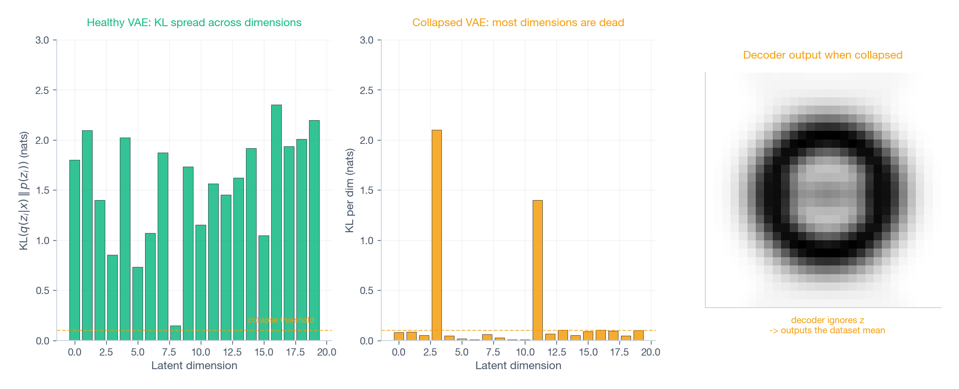
Symptoms. The KL term drops to near zero in the first few epochs and never recovers. Reconstructions look like the average training image regardless of input. Latent traversal produces no visible change.

Root cause. The decoder is powerful enough to reconstruct from $\mu$ alone, or the prior pressure overwhelms the reconstruction signal early in training. The encoder discovers it can satisfy the KL term cheaply by setting $\mu \approx 0,\ \sigma \approx 1$ for every input — i.e., ignoring $x$.

Fixes that work, in order of how often they’re enough:

1. KL annealing. Start at $\beta = 0$ and ramp linearly to 1 over the first 10–20 epochs (the loop above does this). Lets reconstruction get a foothold before KL bites.
2. Free bits. Stop penalizing dimensions whose KL is already small enough — this prevents the optimizer from killing them entirely.

   1 2	kl_per_dim = -0.5 * (1 + logvar - mu.pow(2) - logvar.exp()) kl_loss = torch.sum(torch.clamp(kl_per_dim, min=free_bits))

3. Weaken the decoder. Smaller hidden dim, dropout, or for autoregressive decoders skip the autoregressive shortcut for the first few epochs.

Failure 2: poor sample quality

Symptoms. Reconstructions of training data look fine, but samples drawn as $z \sim \mathcal{N}(0, I)$ are noisy or unrealistic.

Root cause. The aggregated posterior $\frac{1}{N}\sum_i q_\phi(z\mid x_i)$ does not match the prior $p(z)$. There are “holes” in the prior that the decoder never trained on.

Fixes: raise $\beta$ (1.5–4 is common); enlarge the latent ($20 \to 64$); train longer; switch to a stronger decoder (convolutional for images). If you still need photorealism, this is the failure mode that tells you to consider a GAN or diffusion model instead.

Failure 3: blurry reconstructions

Symptoms. Reconstructions are recognizable but smooth and detail-poor; loss plateaus high.

Root cause. Pixel-independent likelihoods (Bernoulli or Gaussian per pixel) penalize only per-pixel error, so the optimum is the conditional mean. That mean is intrinsically blurry under uncertainty.

Fixes: add a perceptual loss (VGG features, LPIPS); switch to a discretized mixture of logistics for natural images; or move to a hierarchical VAE that uses higher-level latents for global structure and lower-level ones for detail.

Failure 4: NaN losses and exploding gradients

Symptoms. Loss becomes NaN after a few hundred steps, or grad norm spikes by orders of magnitude.

Root cause. Almost always one of: unbounded logvar causing exp overflow in the KL; pixel values outside [0, 1] for BCE; learning rate too high; or batch where the reparameterized $\sigma$ underflows.

Fixes:

1
2
3

logvar = torch.clamp(logvar, min=-10, max=10)        # bound exp(logvar)
torch.nn.utils.clip_grad_norm_(model.parameters(), 1.0)
# use AdamW with lr ~1e-3 to 3e-4 and weight_decay ~1e-5

Useful variants

Beta-VAE: explicit disentanglement

Push $\beta$ above 1 to bias the model toward latent dimensions that capture independent factors of variation. The ELBO becomes

with $\beta \in [2, 10]$ typical for disentanglement experiments. The trade-off is exactly what you’d expect: reconstruction degrades as $\beta$ rises.

Conditional VAE: control what gets generated

Condition both encoder and decoder on a label $y$ (digit class, attribute vector, anything):

In code, just concatenate a one-hot $y$ into the encoder input and into $z$ before the decoder. To generate a specific class, sample $z \sim \mathcal{N}(0, I)$ and feed it together with the desired label.

Hierarchical VAE: latents at multiple scales

Stack latents $z_1, z_2, \ldots, z_L$ with $z_{l-1}$ generated conditional on $z_l$. The lower latents capture local detail, the higher ones capture global semantics. Modern variants (NVAE, Very Deep VAE) close most of the sample-quality gap with diffusion using exactly this idea.

Practical tips

1. Normalize your inputs to match your likelihood

BCE expects pixels in $[0, 1]$; Gaussian likelihoods (MSE) work better with zero-centered inputs.

1
2
3
4
5
6
7
8

# MNIST: ToTensor() already gives [0, 1]
transform = transforms.ToTensor()

# Continuous data: standardize to [-1, 1]
transform = transforms.Compose([
    transforms.ToTensor(),
    transforms.Normalize(mean=[0.5], std=[0.5]),
])

2. Start small with the latent

latent_dim = 20 is a reasonable default for MNIST-scale data. Too small bottlenecks reconstruction; too large invites posterior collapse and slows training.

3. Always log reconstruction and KL separately

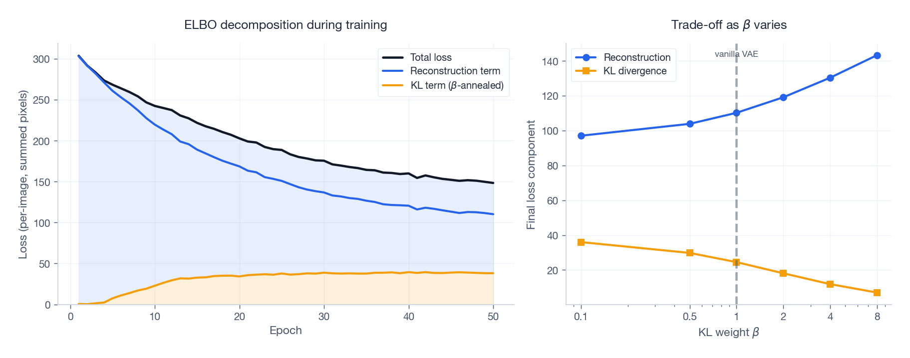
A healthy run shows reconstruction dropping monotonically and KL stabilizing at a non-trivial value (a few nats per active dimension). If KL flatlines at zero you are in posterior collapse; if it explodes, your reconstruction term is being ignored.

4. Visualize the latent space

For a 2-D latent (or after PCA/t-SNE), plot $\mu(x)$ colored by class. You should see overlapping but distinguishable clusters that roughly cover the prior.

 1
 2
 3
 4
 5
 6
 7
 8
 9
10
11
12
13
14

import matplotlib.pyplot as plt

@torch.no_grad()
def plot_latent_space(model, loader, device="cuda"):
    model.eval()
    mus, labels = [], []
    for x, y in loader:
        mu, _ = model.encoder(x.view(-1, 784).to(device))
        mus.append(mu.cpu()); labels.append(y)
    mus    = torch.cat(mus).numpy()
    labels = torch.cat(labels).numpy()
    plt.scatter(mus[:, 0], mus[:, 1], c=labels, cmap="tab10",
                s=8, alpha=0.7)
    plt.colorbar(); plt.title("VAE latent (2D)"); plt.show()

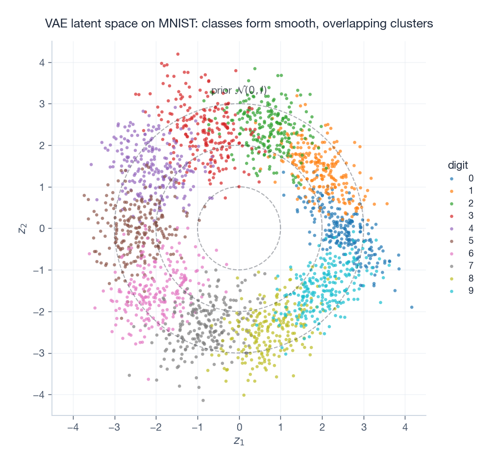
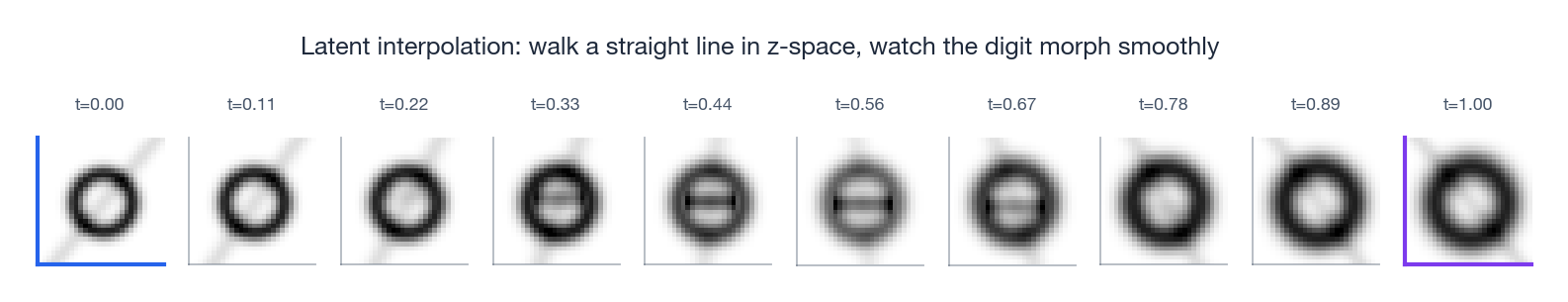
5. Sample, and walk between samples

Two utilities you will reach for constantly:

 1
 2
 3
 4
 5
 6
 7
 8
 9
10
11
12
13
14
15

@torch.no_grad()
def sample_vae(model, n=16, device="cuda"):
    model.eval()
    z = torch.randn(n, model.encoder.fc_mu.out_features).to(device)
    return model.decoder(z).cpu().view(-1, 28, 28)


@torch.no_grad()
def interpolate(model, x1, x2, steps=10, device="cuda"):
    model.eval()
    mu1, _ = model.encoder(x1.view(1, -1).to(device))
    mu2, _ = model.encoder(x2.view(1, -1).to(device))
    ts = torch.linspace(0, 1, steps + 1, device=device).view(-1, 1)
    z  = (1 - ts) * mu1 + ts * mu2
    return model.decoder(z).cpu().view(-1, 28, 28)

A clean interpolation is the single most convincing visual proof that your VAE is actually working.

VAE versus the alternatives

Reach for a VAE when you need an explicit latent representation for downstream tasks, want stable training without adversarial dynamics, or care about disentanglement.

Pick something else when photorealism is the goal (use a GAN or diffusion model), or you only need likelihoods on sequences (use an autoregressive model).

Summary: VAE in five steps

1. Encoder outputs $\mu_\phi(x)$ and $\log \sigma^2_\phi(x)$, not a single deterministic code.
2. Reparameterize: $z = \mu + \sigma \odot \epsilon$ with $\epsilon \sim \mathcal{N}(0, I)$ — gradients now flow.
3. Decoder reconstructs $\hat{x}$ from $z$.
4. Loss = negative ELBO: reconstruction + $\beta$ · KL.
5. Generate: $z \sim \mathcal{N}(0, I) \to$ decoder $\to \hat{x}$.

Hyperparameters that matter most: latent dimension (start at 20), $\beta$ (default 1.0, raise for disentanglement), learning rate (1e-3 with Adam, with KL annealing over 10–20 epochs and grad clipping at 1.0).

Pitfalls to expect: posterior collapse (use KL annealing or free bits), blurry samples (raise latent dim or add perceptual loss), NaN losses (clamp logvar, clip grads).

References

• Kingma, D.P. & Welling, M. (2013). Auto-Encoding Variational Bayes ↗ . The original VAE paper.
• Higgins, I. et al. (2017). beta-VAE: Learning Basic Visual Concepts with a Constrained Variational Framework ↗ .
• Doersch, C. (2016). Tutorial on Variational Autoencoders ↗ . Excellent step-by-step derivation.
• Sohn, K., Lee, H. & Yan, X. (2015). Learning Structured Output Representation using Deep Conditional Generative Models ↗ . The CVAE paper.
• Vahdat, A. & Kautz, J. (2020). NVAE: A Deep Hierarchical Variational Autoencoder ↗ . Hierarchical VAE that competes with GANs on sample quality.
• Kingma, D.P. & Welling, M. (2019). An Introduction to Variational Autoencoders ↗ . Comprehensive monograph.