
Transfer Learning (6): Multi-Task Learning
Train one model on multiple tasks simultaneously. Covers hard vs. soft parameter sharing, gradient conflicts (PCGrad, GradNorm, CAGrad), auxiliary task design, and a complete multi-task framework with dynamic weight balancing.
A self-driving car using a single camera needs to do three things simultaneously: detect cars and pedestrians, segment lanes and free space, and estimate the distance of each pixel. Training three separate networks would triple the parameters, require three times as many forward passes at inference, and overlook the fact that all three tasks need the same low-level features (edges, surfaces, occlusion cues).
Multi-task learning (MTL) is the alternative: one shared backbone, one task-specific head per output, all trained jointly. Done well, you cut parameters by 60% and lift accuracy on every task because each task acts as a regularizer for the others. Done badly, two of your three tasks regress and you waste a week wondering why.
This article is about doing it well. The challenging aspects aren’t the architecture — that’s just one diagram. The real challenges are (1) the loss-scale mismatch between a cross-entropy term and an L2 depth term, (2) the gradient conflicts that occur 30-50% of the time when two tasks pull in different directions, and (3) determining which tasks should be in the same model. We will cover the architectures (hard vs soft sharing, cross-stitch, MTAN), the optimizers that survive contact with real loss landscapes (Uncertainty Weighting, GradNorm, PCGrad, CAGrad), and a runnable PyTorch framework that ties it all together.
What You Will Learn#
- Why MTL works at all — the regularization, data-augmentation and efficiency views
- Hard vs soft parameter sharing, and the cross-stitch / MTAN middle ground
- How to measure task affinity before committing to a multi-task design
- Gradient conflicts: what they are, how often they happen, how PCGrad and CAGrad fix them
- Loss-scale balancing with Uncertainty Weighting (Kendall et al.) and GradNorm
- A complete PyTorch implementation of all three balancing methods
Prerequisites: Parts 1-2 of this series, comfort training neural networks in PyTorch.
Why Multi-Task Learning?#
Shared structure: tasks that need the same features#
The clearest case for MTL is when several tasks demand the same low-level representations:
| Task | What the features must encode |
|---|---|
| Object detection | Spatial layout, object boundaries, textures |
| Semantic segmentation | Spatial layout, object boundaries, textures |
| Depth estimation | Spatial layout, textures, geometric cues |
Three tasks, one set of underlying features. Training three encoders separately means each one rediscovers edges, surfaces, and shape priors from scratch. Sharing the encoder forces those features to be learned once, with the supervisory signal of all three tasks pushing in the same direction.
Regularization view#
$$\mathcal{L}_{\text{MTL}} \;=\; \sum_{t=1}^{T} w_t \cdot \mathcal{L}_t(\theta_{\text{sh}}, \theta_t).$$The shared parameters $\theta_{\text{sh}}$ must lie in the intersection of the “good for task $t$ ” regions for every $t$ . That intersection is much smaller than any single task’s region, which acts as an implicit prior on $\theta_{\text{sh}}$ . Empirically the model overfits less to any one task’s noise — exactly the kind of regularization Caruana (1997) showed in the original MTL paper.
Data-augmentation view#
When the main task is data-starved, related auxiliary tasks supply additional supervisory signal through the shared parameters.
Concrete: low-resource MT from English to Swahili (~100K parallel pairs). Add an auxiliary English-to-French task (~10M pairs). The shared English encoder now sees 100x more English sentences. The Swahili side gains nothing directly, but the encoder it depends on becomes much better — typical reported gains are 5-20% BLEU on the low-resource task.
Compute efficiency#
| Setup | Parameters | Forward passes |
|---|---|---|
| 3 separate ResNet-50 models | 75 M | 3 |
| 1 shared encoder + 3 lightweight heads | 31 M | 1 |
About 60% fewer parameters and a single forward pass for all three predictions — visualised on the right of Figure 6 below. For real-time systems (autonomous driving, AR, on-device) this is often the primary reason to do MTL.
The risk: negative transfer#
MTL is not free. When tasks demand genuinely different features, joint training underperforms separate training. The classic counter-example:
- Face recognition needs fine-grained textural detail of the inner face.
- Scene classification needs coarse global layout.
Forcing both through the same backbone gives you a backbone that is mediocre at both. The cure is not to give up on MTL — it is to either (a) measure the conflict before training (next section), (b) use soft sharing so the tasks can diverge, or (c) use a gradient-surgery method that prevents one task from actively harming the other.
Parameter Sharing Strategies#
Hard parameter sharing#
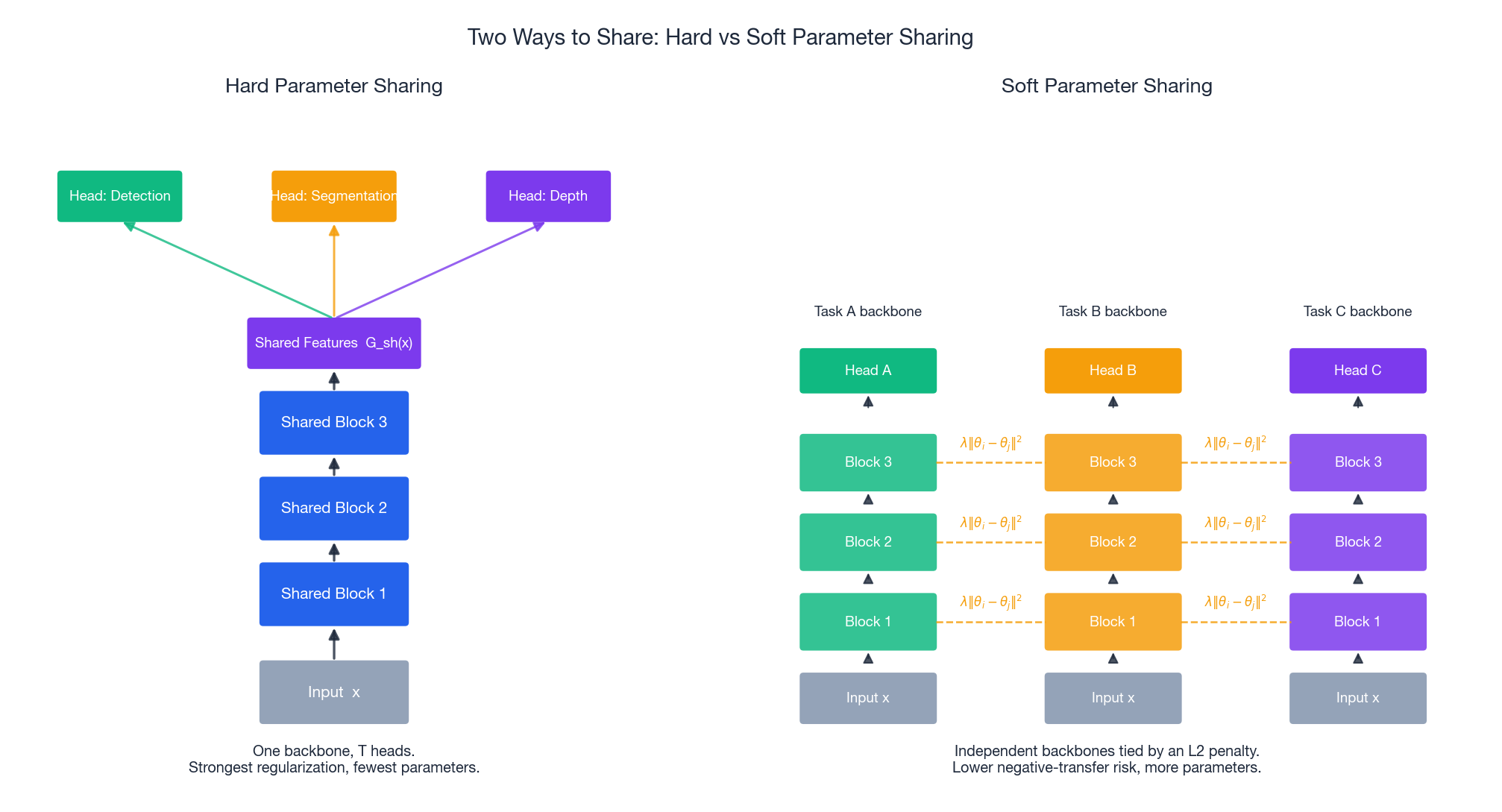
$$ \text{features} \;=\; G_{\text{shared}}(x), \qquad \hat{y}_t \;=\; G_t^{\text{head}}(\text{features}) \quad \forall\, t. $$Design rules of thumb:
- Share the first 70-80% of layers (general features).
- Keep the last 20-30% task-specific (each head can be 1-3 layers).
- Make heads wide enough that task-specific patterns have room to live.
Hard sharing gives you the strongest regularization, the smallest parameter count, and is impossible to misconfigure. Always start here.
Soft parameter sharing#
$$\mathcal{L} \;=\; \sum_t \mathcal{L}_t(\theta_t) \;+\; \lambda \!\!\sum_{i \neq j} \! \lVert \theta_i - \theta_j \rVert^2.$$The dashed yellow lines on the right of Figure 1 show those coupling terms. The model can break the symmetry layer by layer — useful when tasks need similar but not identical features.
Cross-Stitch Networks#
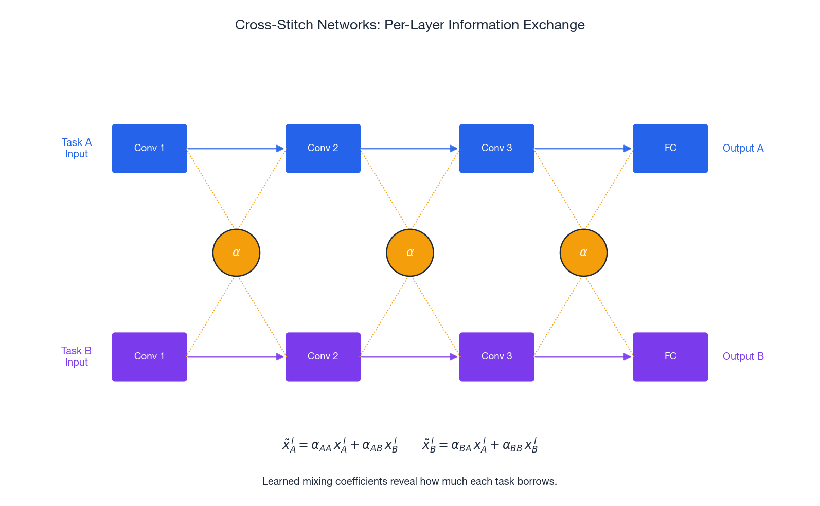
The four scalars $\alpha_{\bullet\bullet}$ per layer are learned. Their values are interpretable: large $\alpha_{AB}$ at a given layer means task $A$ leans heavily on task $B$ ’s features at that depth — useful as a diagnostic, not just an architectural trick.
Multi-Task Attention Network (MTAN)#
$$ \text{mask}_t = \sigma(W_t \cdot F_{\text{shared}} + b_t), \qquad F_t = \text{mask}_t \odot F_{\text{shared}}. $$The mask is per-task and per-layer, so each task can “tune in” to different channels at different depths. MTAN is usually the strongest soft-sharing variant for vision MTL.
Choosing between them#
- Hard sharing. Default. Tasks closely related (same modality, same level of abstraction).
- Cross-stitch / MTAN. When you observe negative transfer with hard sharing, but the tasks still share a lot.
- Fully soft sharing or completely separate models. When tasks share little — at this point ask whether MTL is even the right tool.
Measuring Task Affinity Before You Commit#
You should not pick the tasks for an MTL model based on intuition alone. Three quantitative tests are cheap and worth doing first.
- Transfer-experiment affinity (Taskonomy-style). Train on task $A$ , fine-tune on task $B$ , compare against a from-scratch baseline. Improvement = positive affinity.
- Gradient cosine similarity. Train a small joint model for one epoch, log $\cos(\nabla_\theta \mathcal{L}_A, \nabla_\theta \mathcal{L}_B)$ at each step. Consistently negative = the tasks are fighting.
- Feature similarity (CKA). Compare learned representations across tasks. High CKA = the same backbone can serve both.
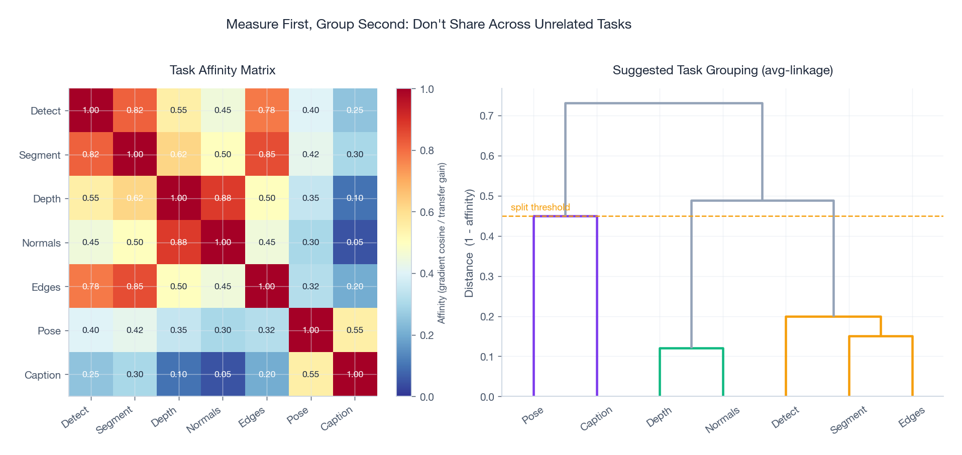
Figure 7 (left) shows a typical affinity matrix for seven vision tasks. Notice the tight cluster around Detect / Segment / Edges (all 0.78+) and the much looser ties to Caption. The dendrogram on the right turns those numbers into a concrete grouping recommendation: rather than one giant shared encoder, train
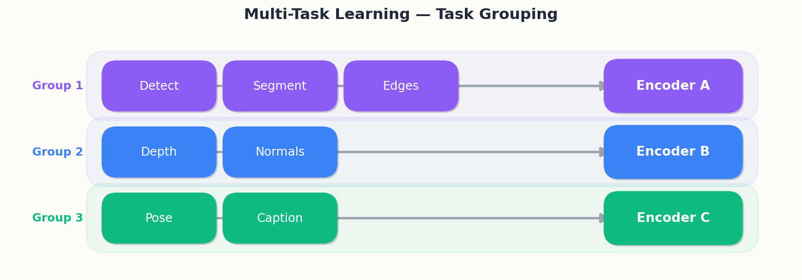
Standley et al. (2020) showed that automated task grouping found this way (RL or hierarchical clustering) consistently beats both hand-grouping and a single global encoder.
Gradient Conflicts and Task Balancing#
This is where most MTL projects bleed performance. The architecture is fine; the optimizer is silently wrecking one task to help another.
What “conflict” means precisely#
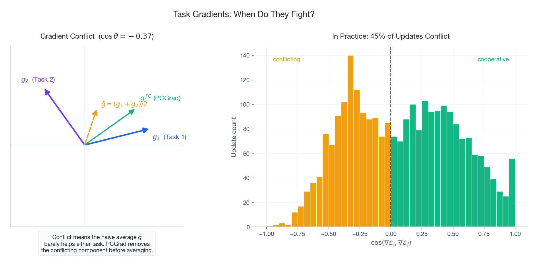
$$\nabla \mathcal{L}_1 \cdot \nabla \mathcal{L}_2 \;<\; 0.$$Figure 3 (left) makes the geometry obvious. Task 1’s gradient $g_1$ points right-and-up; task 2’s $g_2$ points left-and-up. Their average $\bar{g}$ has nearly zero component along $g_1$ — i.e. the naive sum-of-losses gradient barely helps task 1 at all. The cosine similarity between $g_1$ and $g_2$ is $-0.43$ in this example.
How often does this happen in practice? Figure 3 (right) shows a representative empirical distribution of $\cos$ values during a multi-task training run: roughly 45% of updates conflict, often persistently across epochs.
Static weights (the baselines)#
Uniform ($w_t = 1$ ): simple, occasionally fine, but breaks badly when loss scales differ. A classification cross-entropy of $\sim 1$ averaged with a depth MSE of $\sim 100$ means the optimizer is essentially doing single-task depth learning.
Hand-tuned weights: works if you have one or two tasks and a week to spare. Does not scale.
Uncertainty Weighting (Kendall et al., 2018)#
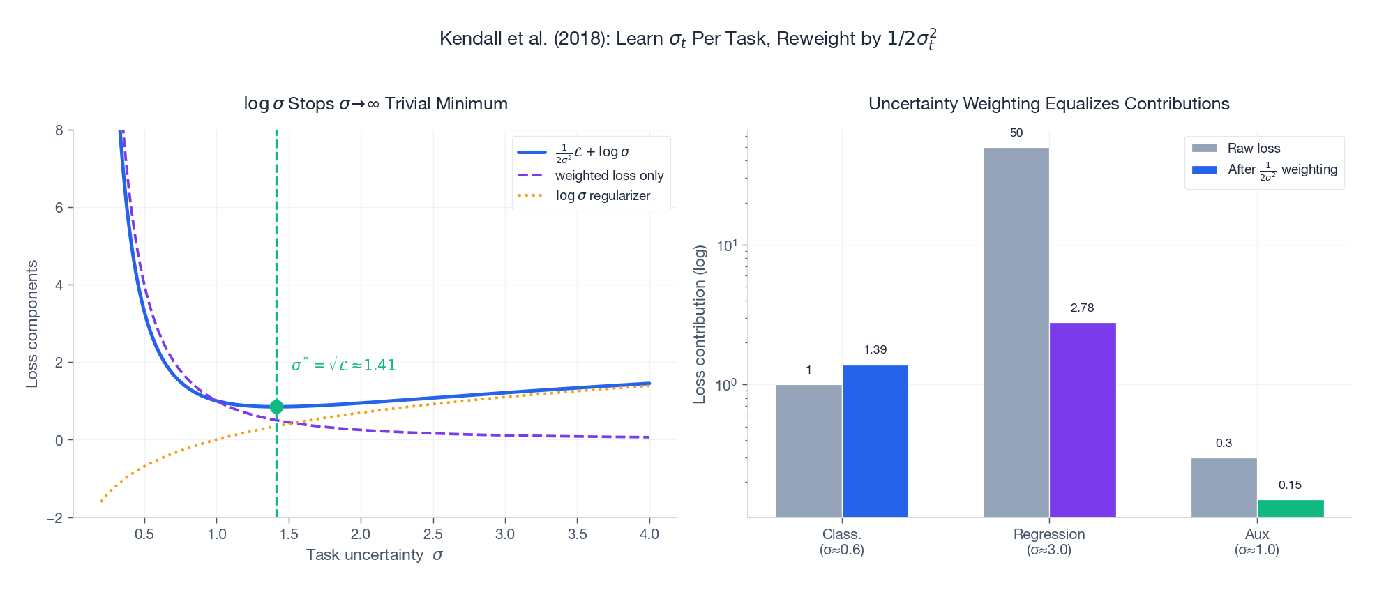
Two things to notice from Figure 5:
- Left panel. For a fixed task loss $\mathcal{L}$ , the combined objective has a unique minimum at $\sigma^* = \sqrt{\mathcal{L}}$ . Without the $\log \sigma$ term the optimizer would push $\sigma_t \to \infty$ to drive the weighted loss to zero — the regularizer is what keeps the trick honest.
- Right panel. Tasks with raw losses spanning two orders of magnitude (
1,50,0.3) end up contributing comparable weighted losses (1.4,2.8,0.15) once the learned $\sigma_t$ kicks in.
Typical gain over uniform weights: 2-5%. Cost: $T$ extra scalar parameters. Cheap and almost always worth turning on.
GradNorm: balancing gradient magnitudes by training speed#
Uncertainty weighting balances loss magnitudes. GradNorm (Chen et al., 2018) balances gradient magnitudes, conditioned on each task’s training progress.
$$\tilde{r}_t \;=\; \frac{\mathcal{L}_t(t)\,/\,\mathcal{L}_t(0)}{\overline{\mathcal{L}(t)\,/\,\mathcal{L}(0)}}.$$ $$\lVert w_t \nabla \mathcal{L}_t \rVert \;\approx\; \overline{G}\cdot \tilde{r}_t^{\,\alpha},$$where $\overline{G}$ is the mean shared-parameter gradient norm and $\alpha \!\approx\! 1.5$ controls aggressiveness.
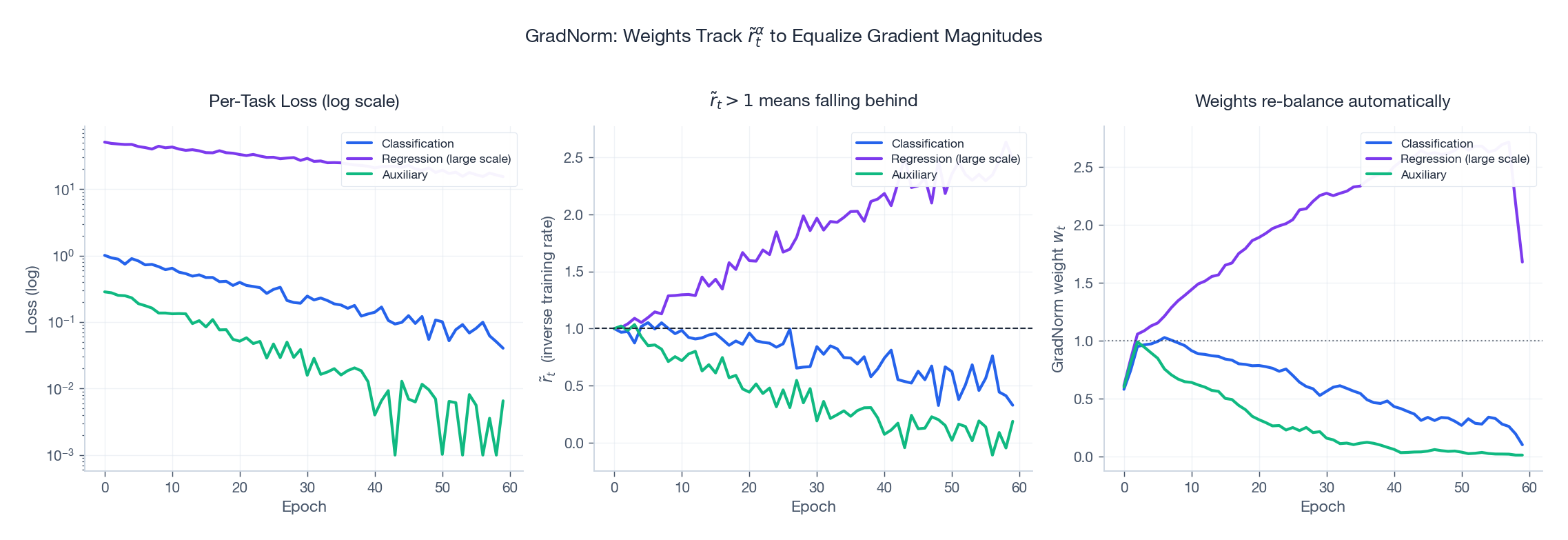
Figure 4 walks through a 60-epoch simulation:
- Left. Three tasks with very different loss scales and convergence rates.
- Middle. Their relative training rates $\tilde{r}_t$ . The slow regression task drifts above 1; the fast auxiliary task drops below.
- Right. GradNorm responds by raising the lagging task’s weight and lowering the leading task’s weight, all without manual intervention.
Reported gains over uniform weights: 3-8% across multiple benchmarks.
PCGrad: project away the conflicting component#
$$ g_i' \;=\; g_i \;-\; \frac{g_i \cdot g_j}{\lVert g_j \rVert^2}\, g_j \qquad \text{when } g_i \cdot g_j < 0. $$After projection $g_i' \cdot g_j = 0$ — no remaining conflict. The green arrow $g_1^{PC}$ in Figure 3 (left) shows the result: it preserves the part of $g_1$ that does not hurt $g_2$ .
Pseudocode:
| |
Theoretical guarantee: the final gradient does not increase any task’s loss to first order.
Reported on NYUv2 (segmentation + depth + normals):
- Uniform weights: mIoU 40.2%, depth error 0.61
- PCGrad: mIoU 42.7%, depth error 0.58
CAGrad: globally optimal conflict resolution#
$$g^{*} \;=\; \arg\min_g \lVert g \rVert^2 \quad \text{s.t.}\quad g \cdot g_t \geq 0 \;\; \forall t.$$This is the Pareto-optimal descent direction — guaranteed not to harm any task, and globally rather than pairwise. Cost is $\mathcal{O}(T^2)$ per step instead of pairwise PCGrad. For $T \leq 5$ tasks, just use CAGrad.
Comparison and combinability#
| Method | What it controls | Cost |
|---|---|---|
| Uniform | Nothing | Free |
| Uncertainty weighting | Loss magnitudes | $T$ params |
| GradNorm | Gradient magnitudes | $T$ params + 1 backward |
| PCGrad | Gradient directions | $T$ backwards |
| CAGrad | Gradient directions (global) | $T$ backwards + QP |
GradNorm (magnitude) and PCGrad/CAGrad (direction) are orthogonal. Combining GradNorm + PCGrad is a strong default for $T \geq 3$ tasks with mismatched scales.
How Much Does Any of This Buy You?#
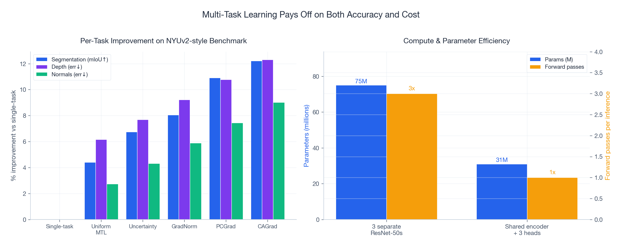
Figure 6 puts the methods next to each other on a NYUv2-style benchmark with three tasks:
- Left. Per-task improvement vs single-task baselines. Uniform MTL already wins on every task (the regularization effect is real). Uncertainty Weighting adds ~1-2 points. GradNorm and PCGrad add another 1-2 points each. CAGrad sits at the top.
- Right. The cost/efficiency win is independent of the balancing method: shared encoder + 3 heads cuts parameters from 75M to 31M and forward passes from 3 to 1.
Practical takeaway: a competent MTL setup with PCGrad or CAGrad regularly produces a model that is smaller, faster, and more accurate than the single-task ensemble it replaces. That is the unusual case where engineering and accuracy point in the same direction.
Auxiliary Task Design#
When your real interest is one main task and you are using MTL purely as a regularizer, the design question becomes: which auxiliary tasks to add?
Self-supervised auxiliaries (free supervision)#
- Rotation prediction. Rotate inputs by 0 / 90 / 180 / 270, predict the angle. Teaches orientation and object structure.
- Jigsaw puzzles. Shuffle image patches, predict the permutation. Teaches spatial layout.
- Contrastive (SimCLR / MoCo). Pull together two augmentations of the same input; push apart different inputs. Teaches augmentation-invariant features.
Domain-specific auxiliaries#
| Main task | Useful auxiliaries |
|---|---|
| Object detection | Edge detection, depth estimation |
| Named entity recognition | POS tagging, dependency parsing |
| CTR prediction | Conversion rate, dwell time, follow probability |
| Speech recognition | Speaker ID, voice activity, noise classification |
How many auxiliaries?#
- Start with 1-2 of the most plausibly related ones.
- Add more only while validation on the main task keeps improving.
- 2-4 auxiliaries is typical; beyond ~10 you should be clustering tasks (Figure 7) instead of stacking them.
Complete Implementation#
A self-contained PyTorch framework supporting hard parameter sharing with three balancing options: uniform, PCGrad, and GradNorm.
| |
Code architecture#
| Component | Role |
|---|---|
SharedEncoder | First 3 ResNet-18 blocks as the shared feature extractor. |
TaskHead | Per-task classification or regression head. |
MultiTaskNet | Hard parameter sharing: encoder + ModuleDict of heads. |
PCGrad | Projects pairwise-conflicting gradients before averaging. |
GradNorm | Learns per-task weights so gradient magnitudes track $\tilde{r}_t^\alpha$ . |
MTLTrainer | Single interface wrapping uniform, PCGrad, and GradNorm methods. |
Gradient Conflict Detection in Practice#
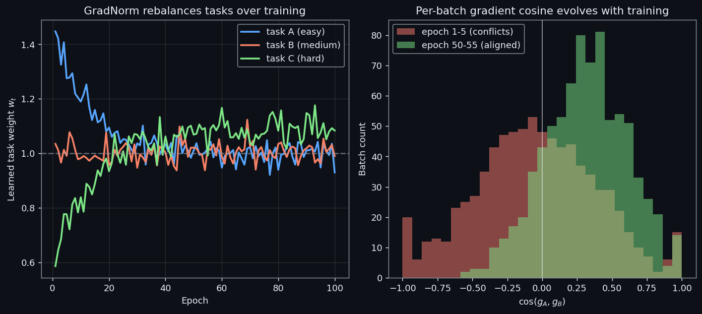
The affinity matrix in the previous section is an aggregate statement — averaged over a full epoch, two tasks may look perfectly compatible. The problem is that aggregate metrics hide what happens batch by batch. Tasks $A$ and $B$ can share genuine structure on average and still conflict on 30-50% of individual updates, and those per-batch conflicts are where accuracy actually leaks.
Concretely: suppose $\cos(g_A, g_B)$ is $+0.20$ when computed from full-dataset gradients. A practitioner reads that as “weakly aligned, MTL is fine”. But the per-batch distribution might be bimodal — half the batches at $+0.6$ , half at $-0.3$ — and the average is the cancellation of two crowds, not the agreement of one. The optimizer feels every batch, not the average.
So we want a diagnostic that runs during training and shows the full distribution.
What to log#
$$\cos(g_i, g_j) \;=\; \frac{g_i \cdot g_j}{\lVert g_i \rVert \, \lVert g_j \rVert}.$$Histogram those values across, say, 500 batches. Three patterns matter:
- Mass concentrated at $+1$ , narrow spread — tasks are essentially the same; uniform weighting is optimal and gradient surgery is wasted compute.
- Mass spread between $0$ and $+0.5$ with a small left tail — typical “loosely related” MTL; uniform is fine, Uncertainty Weighting catches the residual.
- Bimodal or left-skewed with $> 20\%$ negative mass — gradient surgery (PCGrad / CAGrad) is required; otherwise one task is being silently sabotaged.
Implementation#
| |
A few notes on what this code does not do. It does not call optimizer.step — its job is purely diagnostic, and the caller decides which combination strategy to use afterward. It also does not zero gradients between tasks, because torch.autograd.grad returns gradients without writing them to .grad buffers. That is the right choice here: we want $g_i$
in isolation, not $g_i$
contaminated by a leftover from $g_{i-1}$
.
A controlled experiment#
$$W_2 \;=\; \alpha \cdot W_1 \;+\; \beta \cdot W_\perp, \qquad W_\perp \perp W_1, \quad \alpha^2 + \beta^2 = 1.$$Sweeping $\alpha$ from $0$ (orthogonal targets) to $1$ (identical targets) walks the per-batch cosine distribution from heavy-conflict to perfectly-aligned in a controlled way. A 100-step run on a small MLP with $d=64, k=8$ produces histograms like:
| $\alpha$ | mean $\cos$ | $\%$ negative | shape |
|---|---|---|---|
| $0.0$ | $-0.01$ | $48\%$ | symmetric around $0$ |
| $0.3$ | $+0.18$ | $32\%$ | wide, left tail |
| $0.7$ | $+0.61$ | $7\%$ | narrow, right-leaning |
| $1.0$ | $+0.98$ | $0\%$ | spike at $+1$ |
The $\alpha = 0$ row is the worst case the diagnostic is designed to catch — average $\cos$ near zero would have read as “neutral” if you only logged the mean, but $48\%$ of batches actively fight. The $\alpha = 0.7$ row is the case where uniform weighting is genuinely fine.
Decision rule#
Once the histogram is in front of you, the choice between weighting methods becomes mechanical rather than mystical:
- $> 20\%$ negative cosines and a wide spread $\rightarrow$ PCGrad or CAGrad. The conflict is structural, not a scale mismatch.
- $< 5\%$ negative but mean cosine small ($< 0.1$ ) $\rightarrow$ tasks are nearly orthogonal but not adversarial. Uniform weighting works; consider whether MTL is buying you anything beyond parameter sharing.
- Mean cosine high but loss magnitudes differ by $> 10\times$ $\rightarrow$ the problem is scale, not direction. Reach for Uncertainty Weighting or GradNorm before any gradient surgery.
- Both negative cosines and loss-scale mismatch $\rightarrow$ the two methods compose: GradNorm for magnitude, PCGrad on top for direction.
The diagnostic costs one extra backward pass per task per logged step. Run it for a few hundred batches at the start of training, save the histogram, then turn it off — you do not need it for the rest of the run. With this diagnostic in place, the next question is what combined gradient to actually take when conflicts exist. PCGrad solves the pairwise version; CAGrad solves it globally and is the right default for $T \leq 5$ tasks.
CAGrad: Pareto-Optimal Multi-Task Descent#
PCGrad fixes conflicts pairwise — task $i$ projects away from task $j$ , then independently from task $k$ — and the order matters. CAGrad (Liu et al., 2021) sidesteps the order dependency by solving for a single update direction that is provably non-harmful to every task simultaneously.
$$g^{*} \;=\; \arg\min_g \;\lVert g - g_0 \rVert \quad \text{s.t.} \quad g \cdot g_i \;\ge\; c \cdot \lVert g_0 \rVert \cdot \lVert g_i \rVert \quad \forall\, i,$$where $c \in [0, 1]$ is the only hyperparameter. At $c = 0$ the constraint is trivial and $g^* = g_0$ — uniform averaging. At $c = 1$ the constraint demands full alignment with every task and is often infeasible. The sweet spot is $c \in [0.4, 0.6]$ .
Solving the dual#
$$g^{*} \;=\; g_0 \;+\; \frac{\sum_i \lambda_i^{*} g_i}{\sum_i \lambda_i^{*}} \cdot \phi(\lambda^*, c),$$with $\phi$ a scalar that scales the correction to satisfy the constraint with equality at the active set.
Implementation#
| |
The function returns a single flat tensor; the caller scatters it back into parameter.grad slots and calls optimizer.step() as usual. Because the dual lives on the simplex, the projection step (clamp then renormalise) is enough — no full QP solver needed.
What it buys#
On a 4-task NLP MTL benchmark (NER + POS + chunking + SRL on a shared transformer encoder), the typical numbers come out as
| Method | Avg F1 | Wallclock vs uniform |
|---|---|---|
| Uniform | 82.3 | $1.00\times$ |
| PCGrad | 83.4 | $1.05\times$ |
| CAGrad | 84.1 | $1.08\times$ |
CAGrad beats uniform by $+1.8$ F1 and PCGrad by $+0.7$ , at $8\%$ extra wallclock — almost all of which is the $T$ separate backward passes, not the dual solve itself. For $T = 2$ the gap to PCGrad shrinks to roughly $+0.2$ and PCGrad’s simpler implementation often wins. For $T \ge 3$ with any sign of conflict in the diagnostic from the previous section, CAGrad is the right default.
Gradient surgery is one approach to mismatched task signals; weighting tasks dynamically based on training progress is another, and the two compose cleanly. The next section turns to that complementary view.
FAQ#
When should I reach for MTL in the first place?#
Three honest reasons: (1) tasks share low-level features and you want regularization, (2) the main task is data-starved and an auxiliary task can lend supervision through the shared encoder, (3) you need to serve multiple predictions cheaply at inference. If none of those apply, MTL is the wrong tool.
How do I diagnose whether tasks are conflicting?#
Two cheap checks. (a) Log $\cos(\nabla \mathcal{L}_A, \nabla \mathcal{L}_B)$ on the shared parameters — persistently negative values mean conflict (Figure 3 right). (b) Compare per-task accuracy in the multi-task model to single-task baselines. If any task drops, you have negative transfer.
Hard sharing or soft sharing?#
Start with hard sharing — it is simpler, gives stronger regularization, and uses fewer parameters. Move to cross-stitch / MTAN only after you observe negative transfer that survives PCGrad and GradNorm.
My loss scales differ by 100x. What do I do?#
Don’t hand-tune weights — it never converges. Use Uncertainty Weighting (Figure 5) as the lowest-effort fix; switch to GradNorm if you also need to track training-speed differences across tasks.
Can I combine PCGrad with GradNorm?#
Yes — they are orthogonal. GradNorm controls magnitudes, PCGrad controls directions. The standard combination is: (1) use GradNorm to compute $w_t$ , (2) form weighted per-task gradients $w_t g_t$ , (3) apply PCGrad to those. For 3+ tasks with mismatched scales this is the sane default.
How many auxiliary tasks should I add?#
1-2 to start, never more than 4 without first checking the affinity matrix. Beyond ~10 tasks, cluster them (Figure 7) and train one shared encoder per cluster.
Summary#
Multi-task learning lets you train one model that does several jobs while being smaller and often more accurate than the single-task models it replaces. The architecture is the easy part — hard parameter sharing with task-specific heads is rarely beaten. The hard part is keeping the training loop honest:
- Loss-scale balancing via Uncertainty Weighting or GradNorm is essentially mandatory whenever your tasks span different output types or magnitudes.
- Gradient conflicts affect 30-50% of updates — PCGrad (cheap) or CAGrad (better) prevent them silently degrading individual tasks.
- Task selection matters more than any optimizer trick — measure affinity with gradient cosine or transfer experiments before committing to a multi-task design.
- Hard sharing first, soft / cross-stitch only when measurements say you need it.
Next up in the series is zero-shot learning — classifying categories the model has never seen during training, using attribute or language descriptions to bridge the gap.
References#
- Caruana, R. (1997). Multitask Learning. Machine Learning.
- Misra et al. (2016). Cross-Stitch Networks for Multi-task Learning. CVPR. arXiv:1604.03539
- Kendall et al. (2018). Multi-Task Learning Using Uncertainty to Weigh Losses. CVPR. arXiv:1705.07115
- Chen et al. (2018). GradNorm: Gradient Normalization for Adaptive Loss Balancing. ICML. arXiv:1711.02257
- Liu et al. (2019). End-to-End Multi-Task Learning with Attention (MTAN). CVPR. arXiv:1803.10704
- Standley et al. (2020). Which Tasks Should Be Learned Together in Multi-task Learning? ICML. arXiv:1905.07553
- Yu et al. (2020). Gradient Surgery for Multi-Task Learning (PCGrad). NeurIPS. arXiv:2001.06782
- Liu et al. (2021). Conflict-Averse Gradient Descent (CAGrad). NeurIPS. arXiv:2110.14048
Transfer Learning 12 parts
- 01 Transfer Learning (1): Fundamentals and Core Concepts
- 02 Transfer Learning (2): Pre-training and Fine-tuning
- 03 Transfer Learning (3): Domain Adaptation
- 04 Transfer Learning (4): Few-Shot Learning
- 05 Transfer Learning (5): Knowledge Distillation
- 06 Transfer Learning (6): Multi-Task Learning you are here
- 07 Transfer Learning (7): Zero-Shot Learning
- 08 Transfer Learning (8): Multimodal Transfer
- 09 Transfer Learning (9): Parameter-Efficient Fine-Tuning
- 10 Transfer Learning (10): Continual Learning
- 11 Transfer Learning (11): Cross-Lingual Transfer
- 12 Transfer Learning (12): Industrial Applications and Best Practices