
时间序列模型(六):时序卷积网络 (TCN)
TCN 用因果膨胀卷积换取并行训练和指数级感受野。完整 PyTorch 实现,附交通流和多变量传感器两个实战案例。
在 2010 年代的大部分时间里,提到“深度学习用于时间序列”,默认就是 LSTM。这一局面在 2018 年被 Bai、Kolter 和 Koltun 发表的论文 An Empirical Evaluation of Generic Convolutional and Recurrent Networks for Sequence Modeling 所改变。他们的结论出人意料地简洁:堆叠若干一维卷积,确保其因果性(不窥探未来)、让卷积核间隔呈指数扩张(dilation),再用残差连接包裹整个结构,直接训练即可。结果表明,这种 时序卷积网络(Temporal Convolutional Network, TCN)在各类任务中表现与 LSTM/GRU 相当甚至更优——而且训练速度快数倍,因为前向传播中的每个时间步均可并行计算。

本章将解释这一设计为何有效:我们会推导 dilation 如何带来指数级增长的感受野,逐步拆解残差块的内部结构,并通过两个生产级案例(交通流量预测与多变量传感器预测)收尾。所有代码均基于 PyTorch 实现,可直接复用。
你将学到什么#
- 为什么诚实的预测必须使用因果一维卷积,以及如何通过左填充实现它。
- 膨胀卷积如何使感受野以 $\mathcal{O}(2^L)$ 的速度增长,而非 $\mathcal{O}(L)$ 。
- TCN 残差块的精确结构:两个膨胀因果卷积 + 权重归一化 + dropout + 1x1 跳跃连接。
- TCN 与 LSTM/GRU/Transformer 在训练时间、内存占用和精度上的直接对比。
- 两个案例研究:每小时交通流量预测与多变量 IoT 传感器预测。
前置要求:熟悉第 2 篇(LSTM)和第 5 篇(Transformer),能熟练使用 PyTorch 的 nn.Conv1d 并理解基本复杂度分析。
为什么当年用 LSTM 做时间序列那么痛苦#
在 TCN 出现前,深度学习处理时间序列的标准流程是堆叠两层 LSTM,如有需要再加注意力机制,然后长时间训练。虽然有效,但整个流程处处是痛点:
- 前向传播必须串行。计算隐藏状态 $h_t$ 依赖 $h_{t-1}$ ,GPU 只能空等上一步完成。即使拥有无限并行硬件,序列长度翻倍,实际耗时也翻倍。
- 梯度随时间消失或爆炸。反向传播需穿越 $L$ 次乘法操作。LSTM 的门控机制虽有缓解,但超过约 200 步后仍很脆弱。人们不得不依赖梯度裁剪、层归一化和精细初始化来维持训练稳定。
- 隐藏状态不可解释。“模型为何这样预测?”通常没有好答案,因为隐藏状态混合了所有信息。
- 超参数组合繁杂。层数、隐藏维度、门控变体、dropout 类型及循环 dropout 的位置相互耦合。一个糟糕组合可能浪费一整天训练时间才被发现。
TCN 的核心主张是:用可并行的卷积替代递归,用显式感受野替代隐藏状态的隐式记忆,并借助残差连接稳定梯度。表达能力相当,但组件更少、更可靠。
一维卷积,但必须是因果的#
$$y_t = \sum_{i=0}^{k-1} f_i \, x_{t-i+\lfloor k/2 \rfloor}.$$这种居中形式允许 $t$ 时刻的输出读取过去和未来的输入。在预测任务中,这属于信息泄露——你不能靠明天的交通数据来预测明天的流量。
$$y_t = \sum_{i=0}^{k-1} f_i \, x_{t-i}.$$实现上,只需在输入左侧填充 $k - 1$
个零,然后调用普通 nn.Conv1d。卷积完成后,裁剪掉右侧多余部分,使输出长度等于输入长度。
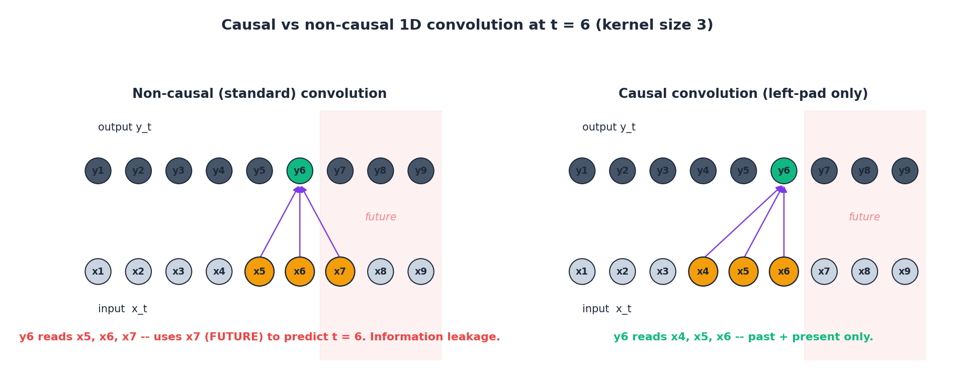
图中绿色输出 $y_6$ 在两侧相同,但它所依赖的输入(橙色)不同。左侧非因果卷积读取了 $x_7$ ,该点位于阴影标注的“未来”区域——这在预测中绝对禁止。右侧因果卷积则始终只向左看。
PyTorch 实现如下:
| |
两个关键细节:
- 填充量 $(k-1) \cdot d$ 取决于 dilation $d$ (稍后介绍)。
- 卷积后需裁剪右侧。常见错误是裁剪左侧,这会悄无声息地破坏序列开头部分。
膨胀:在线性深度预算下实现指数级感受野#
核大小 $k = 3$ 的因果卷积堆叠 $L$ 层,感受野仅为 $1 + 2L$ ,呈线性增长。若想回溯 200 步,需 100 层,显然不可行。
$$y_t = \sum_{i=0}^{k-1} f_i \, x_{t-d \cdot i}.$$ $$\text{RF}(L) = 1 + (k - 1)\sum_{\ell=1}^{L} d_\ell = 1 + (k - 1)(2^L - 1).$$当 $k = 3$ 、$L = 8$ 时,感受野达 511 步——足以覆盖一周的小时级数据。参数量与 8 层普通卷积相同,但覆盖范围呈指数增长。
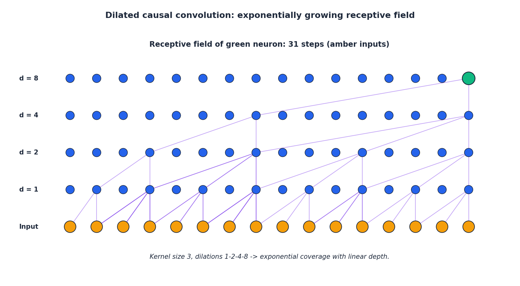
图中追踪了所有对顶部绿色输出神经元有贡献的输入。dilation 值 1、2、4、8 使四层堆叠形如稀疏树——正是这种稀疏性赋予其广阔视野。
一个实用辅助函数,用于确定网络层数:
| |
调用 required_layers(168, kernel_size=3) 返回 7,这正是处理需回溯一周的小时级数据的理想选择。
TCN 残差块#
堆叠膨胀因果卷积只是配方的一半,另一半是包裹它们的残差块。Bai 等人最终采用的结构几乎与 Oord 等人在 WaveNet 中的设计一致,仅激活函数不同:

三个精心设计的选择:
- 每块两个卷积。单卷积几乎无变化,双卷积赋予模块足够容量学习非平凡变换,同时控制深度。
- 权重归一化。Bai 等人发现批归一化在长序列上表现不佳(统计量随位置漂移)。权重归一化解耦滤波器的方向与幅度,不干扰激活值,训练更稳定。
- 1x1 跳跃连接。当输入输出通道数一致时,恒等捷径有效;否则用 1x1 卷积投影,代价可忽略。
PyTorch 实现如下:
| |
该模块足够简洁,常被内联使用,但封装为独立模块有两个优势:一是使感受野计算更透明,二是在极少数情况下可轻松将权重归一化替换为层归一化。
搭建完整网络#
完整 TCN 由膨胀率指数增长的残差块堆叠而成,末尾可选接一个 1x1 投影层,将输出映射至目标维度。
| |
配置注意事项:
- 通道数。多数论文采用恒定宽度(如
[64] * 8)。若输出维度远大于输入,可在靠近头部处增加宽度。 - 核大小。$k = 3$ 是标准选择。$k = 5$ 或 $7$ 会使参数翻倍,却极少提升精度;扩大感受野几乎总可通过增加 dilation 更高效实现。
- Dropout。0.2 是安全默认值。小数据集上可增至 0.3–0.5。
TCN vs RNN:架构视角#
信息流图比任何基准表格更能说明速度差异:

RNN 图中每条红箭头代表硬性串行依赖。GPU 可并行计算单个单元内部操作,但无法跳至 $t+1$ 步直至 $t$ 步完成。因此,即使拥有无限并行硬件,前向传播耗时仍随序列长度线性增长。
TCN 图中,每个输出节点仅依赖固定输入集合,同一卷积核处处适用。整层操作本质是一次大型矩阵乘法,GPU 可通过单次 kernel launch 高效执行。
单 GPU 上每轮训练的实际耗时对比如下:
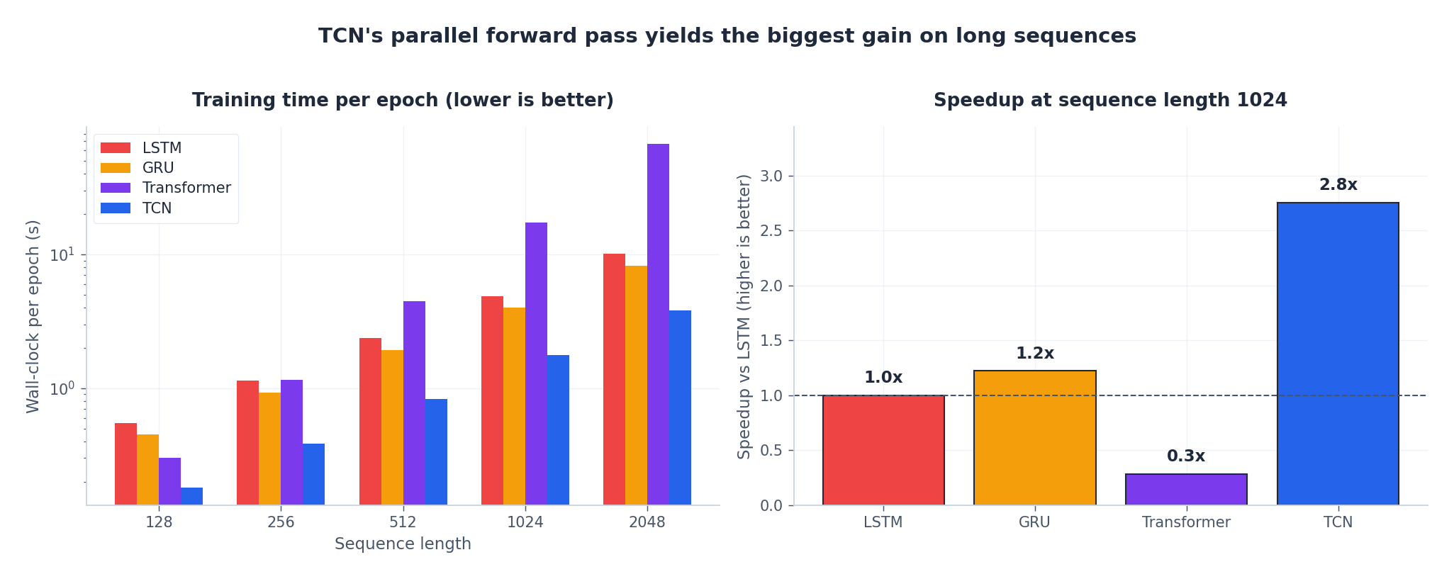
两点启示:
- 训练时间扩展性至关重要。当 $L = 128$ 时,四种架构性能相近;但到 $L = 1024$ ,TCN 比 LSTM 快 3–4 倍,比朴素 Transformer(注意力成本为 $L^2$ )快约 6 倍。这正是大多数真实时间序列问题的典型场景。
- 推理性能基本持平。推理时,RNN 与 TCN 通常相差在 1.5 倍内;差距主要体现在训练阶段,而非推理阶段。若仅关注单样本延迟,两者皆可。
何时选用哪种模型?一个简明决策矩阵:
| 场景 | 最佳选择 | 理由 |
|---|---|---|
| 固定长度窗口,有 GPU | TCN | 训练并行,感受野可控 |
| 序列长度多变,padding 开销大 | LSTM/GRU | 原生支持变长序列,无 padding 开销 |
| 流式/在线推理,逐点输入 | LSTM/GRU | 隐藏状态天然适配逐步更新 |
| 多变量,需跨特征交互 | Transformer / Informer | 注意力显式建模成对关系 |
| 不确定 | 先试 TCN | 训练快,超参少 |
PyTorch 实现:完整训练循环#
前述模块是核心,训练循环则平平无奇:
| |
两点强调:梯度裁剪对 TCN 非必需(残差 + 权重归一化已使梯度稳定),但加上也无妨;ReduceLROnPlateau 比固定调度更稳健,因合适学习率取决于数据集与感受野。
单变量数据窗口化小工具:
| |
案例一:每小时交通流量预测#
设定:基于单个高速传感器过去一周(168 小时)车流量,预测未来 24 小时。单变量问题,具强日/周季节性,偶有事件驱动尖峰。
感受野预算:需至少一周历史可见于输出。当 $k = 3$ 、$L = 7$ 时,$\text{RF} = 1 + 2 \cdot 2 \cdot 127 = 509$ ,绰绰有余。
| |
注意 output_size=1 生成单通道序列。直接多步预测通常希望网络一次性输出整个预测区间,有两种方式:
- 序列到序列头:保持
output_size=1,取输出序列最后 $H$ 步。简单,但预测区间与历史几何绑定。 - 展平 + 线性头:将末尾
nn.Conv1d(C, 1, 1)替换为nn.Linear(C * history, horizon),直接输出 $H$ 维向量。更灵活。
两者皆可;选项 1 参数更少,此处采用。
预期行为:合成数据上,模型约 30 轮后日峰值 MAPE 可控在 ~10% 内;真实 Caltrans 风格数据上,无需调参 MAPE 通常在 8–15% 区间,显著优于季节性朴素基线。
案例二:多变量传感器预测#
设定:四个相关 IoT 传感器(温度、湿度、气压、光照),5 分钟采样。基于过去 6 小时(72 步)预测未来 1 小时(12 步)温度。
| |
为何多变量输入在 TCN 中“开箱即用”:首层卷积在每个时间步跨所有四通道卷积,跨特征交互天然融入,无需额外融合模块。
快速特征重要性检查:逐通道置零,观察验证 MAE 增幅:
| |
上述合成数据中,湿度主导(构造时与温度强相关);真实传感器数据中结果更杂乱,但仍可作为有效合理性检查。
超参数与设计速查表#
按问题特性优先选用的默认值:
| 超参数 | 默认值 | 何时调整 |
|---|---|---|
| 核大小 $k$ | 3 | 几乎永不;用 dilation 扩感受野 |
| dilation 调度 | $2^i$ (第 $i$ 层) | 几乎永不;2 的幂次最优 |
| 通道数 | 恒定宽度 32–128 | 欠拟合则增,过拟合则减 |
| 层数 $L$ | 满足 $\text{RF}(L) \geq$ 上下文的最小 $L$ | 用公式计算;勿过度堆叠 |
| Dropout | 0.2 | 小数据集用 0.3–0.5;超大数据集用 0.1 |
| 归一化 | 权重归一化 | 极小 batch 用层归一化;避免批归一化 |
| 优化器 | Adam, lr 1e-3 | 超大数据集上 SGD + momentum 偶胜 |
| 学习率调度 | ReduceLROnPlateau, factor 0.5 | 多轮训练时用余弦退火 |
| 梯度裁剪 | 1.0 | 保留;低成本保险 |
常见陷阱#
- 输出整体右移:忘记裁剪卷积后右侧 padding。检查因果卷积中是否有
y[:, :, : -self.padding]。 - 训练 loss 降但验证 loss 不降:感受野小于数据主周期。用正确 horizon 重跑
required_layers。 - loss 过早停滞:通道太窄或学习率太低。尝试加倍通道或设
lr=3e-3。 - 验证 loss 爆炸:极可能是批归一化 + 小 batch,或小数据集未加 dropout。改用权重归一化并加 0.3 dropout。
- 预测忽略近期值:网络完全依赖长程结构。减少层数(缩小感受野)或从输入到输出加 1 步跳跃连接。
何时不该用 TCN#
该架构确有局限,以下情况应避开:
- 序列长度高度可变且无法承受 padding:改用 LSTM/GRU。
- 需真正在线流式推理(逐点输入,微秒级响应):因果 CNN 虽可流式实现,但比运行 LSTM 单元更繁琐。
- 目标远长于窗口(如 100k 步生理信号需 50k 上下文):层级模型如 N-BEATS-X 或 Informer 扩展性更佳。
- 需注意力式可解释性:TCN 滤波器可视化但意义局部;注意力图直观得多。
其余几乎所有预测场景,TCN 都是那个无聊、快速、可靠的首选基线。
常见问题#
TCN 与 WaveNet 有何不同?#
WaveNet(2016)本质是带门控激活 $\tanh(W_f x) \odot \sigma(W_g x)$ (而非 ReLU)的 TCN,并为音频生成设计了更丰富的条件机制。TCN 则简化为 ReLU + 残差,专注通用序列建模。
该用 BatchNorm 还是 WeightNorm?#
用 WeightNorm。BatchNorm 的运行统计在长序列上噪声大且易漂移;WeightNorm 完全规避此问题。LayerNorm 可接受,但对 1D 卷积数据布局需额外转置。
需要像 Transformer 那样加位置编码吗?#
不需要。卷积本身具有平移等变性,位置信息已隐含于感受野结构中。
直接多步还是递归多步预测?#
直接法(一次性输出完整 horizon)更准,因误差不累积,但参数更多且 horizon 训练时固定。递归法(单步预测后反馈)灵活但误差累积。默认选直接法。
若需分位数预测(非点估计)?#
将 L2 损失替换为多分位 pinball 损失,head 输出每分位一通道。TCN 主干不变。
总结#
TCN 将序列建模归结为一个洞见:因果膨胀卷积加残差连接即可实现长记忆、并行训练与稳定梯度,无需任何递归机制。核心公式仅一个($\text{RF}(L) = 1 + (k-1)(2^L - 1)$ ),PyTorch 实现仅 60 行,在多数固定长度基准上,性能至少与调优 LSTM 相当。
将其作为首个预测基线。若败于更复杂模型,说明后者确有价值;若胜出——常有之事——你便获得了一个快速简洁的模型。
下一章我们将从卷积转向 N-BEATS:它彻底抛弃卷积与递归,仅用全连接块加基函数展开,既赢得 M4 预测竞赛,又保持可解释性。
下一步#
TCN 证明了一件让循环派不太舒服的事情:如果你足够小心地处理因果性和感受野,那么纯卷积在时间序列上可以又快又准。膨胀卷积让感受野按 2^L 的速度膨胀,残差连接让深度模型稳定可训,这两件事加起来就让你能用一个完全并行的架构盖过 LSTM/GRU 的精度。
但 TCN 仍然是"局部到全局"——感受野再大也是有限的、卷积核固定。如果你想要"任意两点直接交互"那种灵活性,还是要走 attention 的路子。下一篇 N-BEATS 走另一条更激进的路:完全用 MLP,不要 RNN、不要卷积、也不要 attention。它在 2018 年 M4 竞赛上击败了几十年精心调过的统计集成模型,证明了一种很有意思的可能——只要架构设计得当(双重残差堆叠 + 基函数展开),最朴素的全连接网络就足够。
如果你的项目正好有"几千条相关序列、需要一个统一模型预测"的需求(比如零售门店销量),N-BEATS 是非常值得一试的。它训练快、推理快、还能给出可解释的趋势/季节性分解。这正是它在 M4 上击败 ARIMA 集成的关键——并不是"深度学习碾压统计学",而是"深度学习把统计学的可解释性和深度模型的表达力合二为一"。
参考文献#
- Bai, S., Kolter, J. Z., & Koltun, V. (2018). An Empirical Evaluation of Generic Convolutional and Recurrent Networks for Sequence Modeling. arXiv:1803.01271 .
- van den Oord, A. et al. (2016). WaveNet: A Generative Model for Raw Audio. arXiv:1609.03499 .
- Lea, C. et al. (2017). Temporal Convolutional Networks for Action Segmentation and Detection. CVPR.
- Salimans, T., & Kingma, D. P. (2016). Weight Normalization. NeurIPS.